[DL101] Chương 4: Thị giác máy tính sử dụng Mạng nơ-ron tích chập (CNNS)

Bài viết có tham khảo, sử dụng và sửa đổi tài nguyên từ kho lưu trữ handson-mlp, tuân thủ giấy phép Apache‑2.0. Chúng tôi chân thành cảm ơn tác giả Aurélien Géron (@aureliengeron) vì sự chia sẻ kiến thức tuyệt vời và những đóng góp quý giá cho cộng đồng.

Ở chương này, chúng ta sẽ tìm hiểu về Thị giác Máy tính (Computer Vision) và Mạng nơ-ron Tích chập (Convolutional Neural Networks - CNNs).

Không giống như các chương trước làm việc với dữ liệu dạng bảng hay vector đơn giản, hình ảnh là dữ liệu có cấu trúc không gian đặc biệt. CNN được thiết kế để tận dụng chính cấu trúc này thông qua cơ chế chia sẻ trọng số (parameter sharing) và kết nối cục bộ (local connectivity). Điều này không chỉ giúp giảm đáng kể số lượng tham số cần huấn luyện mà còn mang lại tính chất quan trọng: bất biến tịnh tiến (translation invariance).

Chương này sẽ trang bị cho bạn:

Nền tảng toán học: Từ phép tích chập (convolution) đến cơ chế gộp (pooling).
Kỹ năng thực hành: Xây dựng CNN từ con số 0 và sử dụng các mô hình tiên tiến như ConvNeXt.
Ứng dụng đa dạng: Từ phân loại ảnh (Classification) đến định vị (Localization) và phát hiện đối tượng (Object Detection) với YOLO.

Bạn có thể chạy trực tiếp các đoạn mã code tại: Google Colab.

Cài đặt môi trường (Setup)

Chúng ta cần đảm bảo môi trường thực thi được kiểm soát chặt chẽ.

Kiểm tra phiên bản Python:

import sys

# Kiểm tra phiên bản Python, yêu cầu >= 3.10
assert sys.version_info >= (3, 10)

Xác định môi trường thực thi để cấu hình phù hợp:

IS_COLAB = "google.colab" in sys.modules
IS_KAGGLE = "kaggle_secrets" in sys.modules

Cài đặt thư viện TorchMetrics để tính toán các chỉ số đánh giá chuẩn xác:

if IS_COLAB:
    %pip install -q torchmetrics

output:
     [?25l    [90m━━━━━━━━━━━━━━━━━━━━━━━━━━━━━━━━━━━━━━━━ [0m  [32m0.0/983.2 kB [0m  [31m? [0m eta  [36m-:--:-- [0m
 [2K    [91m━━━━━━━━━━━━━━━━━━━━━━━━━━━━━━━━━━━━━━━ [0m [91m╸ [0m  [32m983.0/983.2 kB [0m  [31m37.8 MB/s [0m eta  [36m0:00:01 [0m
 [2K    [90m━━━━━━━━━━━━━━━━━━━━━━━━━━━━━━━━━━━━━━━━ [0m  [32m983.2/983.2 kB [0m  [31m26.6 MB/s [0m eta  [36m0:00:00 [0m
     [?25h

Kiểm tra phiên bản PyTorch (yêu cầu tối thiểu 2.6.0 để hỗ trợ các kiến trúc mới):

from packaging.version import Version
import torch

assert Version(torch.__version__) >= Version("2.6.0")

Cấu hình phần cứng: CNN thực hiện hàng tỷ phép tính nhân ma trận. GPU là bắt buộc để huấn luyện hiệu quả.

if torch.cuda.is_available():
    device = "cuda"
elif torch.backends.mps.is_available():
    device = "mps"
else:
    device = "cpu"

device

output:
    'cuda'

Cảnh báo nếu không có GPU:

if device == "cpu":
    print("Neural nets can be very slow without a hardware accelerator.")
    if IS_COLAB:
        print("Go to Runtime > Change runtime and select a GPU hardware "
              "accelerator.")
    if IS_KAGGLE:
        print("Go to Settings > Accelerator and select GPU.")

Cấu hình hiển thị biểu đồ:

import matplotlib.pyplot as plt

plt.rc('font', size=14)
plt.rc('axes', labelsize=14, titlesize=14)
plt.rc('legend', fontsize=14)
plt.rc('xtick', labelsize=10)
plt.rc('ytick', labelsize=10)

Các lớp Tích chập (Convolutional Layers)

Cơ sở lý thuyết

Phép toán Tích chập

Về mặt toán học, phép tích chập 2D rời rạc giữa ảnh đầu vào $I$ và hạt nhân (kernel/filter) $K$ kích thước $k \times k$ được định nghĩa: $(I * K)(i, j) = \sum_{m=0}^{k-1} \sum_{n=0}^{k-1} I(i-m, j-n) K(m, n)$ Tuy nhiên, trong các thư viện Deep Learning (như PyTorch), phép toán thực sự được cài đặt là tương quan chéo (cross-correlation), không có bước lật ngược kernel: $(I \star K)(i, j) = \sum_{m=0}^{k-1} \sum_{n=0}^{k-1} I(i+m, j+n) K(m, n)$ Sự khác biệt này không ảnh hưởng đến khả năng học của mạng vì trọng số $K$ được học từ dữ liệu.

Công thức tổng quát cho một lớp tích chập với nhiều kênh đầu vào và đầu ra: Cho đầu vào $X \in \mathbb{R}^{C_{in} \times H \times W}$ và bộ lọc $W \in \mathbb{R}^{C_{out} \times C_{in} \times K_H \times K_W}$ . Đầu ra $Y \in \mathbb{R}^{C_{out} \times H' \times W'}$ tại vị trí $(c, h, w)$ là: $Y_{c,h,w} = b_c + \sum_{k=0}^{C_{in}-1} \sum_{u=0}^{K_H-1} \sum_{v=0}^{K_W-1} X_{k, h \cdot s + u, w \cdot s + v} \cdot W_{c, k, u, v}$ Trong đó $s$ là bước trượt (stride) và $b$ là bias.

Thực hành: Triển khai Lớp Tích chập với PyTorch

import numpy as np
import torch
from sklearn.datasets import load_sample_images

# Tải ảnh mẫu (định dạng numpy array)
sample_images = np.stack(load_sample_images()["images"])

# Chuyển đổi sang tensor và chuẩn hóa giá trị pixel về khoảng [0, 1]
sample_images = torch.tensor(sample_images, dtype=torch.float32) / 255

# Kiểm tra kích thước của tensor ảnh gốc
# Định dạng hiện tại: [batch_size, height, width, channels]
sample_images.shape

output:
    torch.Size([2, 427, 640, 3])

PyTorch yêu cầu định dạng [batch, channels, height, width] (NCHW), tối ưu cho tính toán GPU.

# Hoán đổi trục: chuyển channels (trục 3) lên vị trí thứ 2 (trục 1)
sample_images_permuted = sample_images.permute(0, 3, 1, 2)
sample_images_permuted.shape

output:
    torch.Size([2, 3, 427, 640])

# Hàm hỗ trợ hiển thị ảnh
def plot_image(image):
    # Khi hiển thị bằng matplotlib, cần chuyển lại về [height, width, channels]
    plt.imshow(image.permute(1, 2, 0))
    plt.axis("off")

plt.figure(figsize=(8, 4))
for index, image in enumerate(sample_images_permuted):
    plt.subplot(1, 2, index + 1)
    plot_image(image)

alt text

Cắt ảnh để tập trung vào chi tiết:

import torchvision
import torchvision.transforms.v2 as T

# Cắt ảnh tại trung tâm, kích thước 70x120
cropped_images = T.CenterCrop((70, 120))(sample_images_permuted)
cropped_images.shape

output:
    torch.Size([2, 3, 70, 120])

plt.figure(figsize=(8, 4))
plt.subplot(1, 2, 1)
plot_image(cropped_images[0])
plt.subplot(1, 2, 2)
plot_image(cropped_images[1])

alt text

Tạo lớp Conv2d:

import torch.nn as nn

torch.manual_seed(42) # Cố định seed để tái lập kết quả

# Tạo lớp Conv2d: vào 3 kênh, ra 32 kênh, kích thước kernel 7x7
conv_layer = nn.Conv2d(in_channels=3, out_channels=32, kernel_size=7)

# Cho ảnh đi qua lớp tích chập
fmaps = conv_layer(cropped_images)

Kích thước đầu ra được tính: $H_{out} = \lfloor \frac{H_{in} + 2 \times \text{padding} - \text{kernel\_size}}{\text{stride}} + 1 \rfloor$ . Ở đây: $H_{out} = \lfloor \frac{70 + 0 - 7}{1} + 1 \rfloor = 64$ .

# Kích thước đầu ra: [batch, out_channels, height_out, width_out]
# Lưu ý kích thước giảm đi do không dùng padding
fmaps.shape

output:
    torch.Size([2, 32, 64, 114])

# Hiển thị 2 feature maps đầu tiên của mỗi ảnh
plt.figure(figsize=(8, 4))
for image_idx in (0, 1):
    for fmap_idx in (0, 1):
        plt.subplot(2, 2, image_idx * 2 + fmap_idx + 1)
        # .detach() để tách tensor khỏi đồ thị tính toán trước khi vẽ
        plt.imshow(fmaps[image_idx, fmap_idx].detach(), cmap="gray")
        plt.axis("off")

plt.show()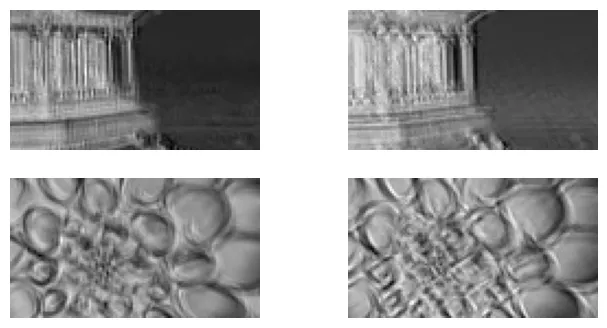

alt text

Padding và Stride

# Sử dụng padding="same" để giữ nguyên kích thước không gian
conv_layer = nn.Conv2d(in_channels=3, out_channels=32, kernel_size=7,
                       padding="same")
fmaps = conv_layer(cropped_images)
fmaps.shape # Kích thước 70x120 được bảo toàn

output:
    torch.Size([2, 32, 70, 120])

# Sử dụng stride=2 sẽ làm giảm một nửa kích thước chiều cao và chiều rộng
conv_layer = nn.Conv2d(in_channels=3, out_channels=32, kernel_size=7, stride=2,
                       padding=3)
fmaps = conv_layer(cropped_images)
fmaps.shape

output:
    torch.Size([2, 32, 35, 60])

Kích thước trọng số:

# [out_channels, in_channels, kernel_height, kernel_width]
conv_layer.weight.shape

output:
    torch.Size([32, 3, 7, 7])

# Mỗi feature map đầu ra có 1 bias
conv_layer.bias.shape

output:
    torch.Size([32])

Thao tác thủ công với Bộ lọc

Minh họa cách bộ lọc phát hiện cạnh dọc và ngang.

import torch.nn.functional as F

# Tạo bộ lọc thủ công
torch.manual_seed(42)
filters = torch.randn([2, 3, 7, 7]) # 2 filters, 3 channels, 7x7 size
biases = torch.zeros([2])

# Sử dụng hàm F.conv2d để thực hiện phép tích chập trực tiếp mà không cần tạo lớp nn.Conv2d
fmaps = F.conv2d(cropped_images, filters, biases, stride=1, padding="same")
fmaps.shape

output:
    torch.Size([2, 2, 70, 120])

plt.figure(figsize=(8, 4))

# Khởi tạo 2 bộ lọc với toàn số 0
filters = torch.zeros([2, 3, 7, 7])

# Bộ lọc 0: Đường dọc ở cột thứ 3
filters[0, :, :, 3] = 1
# Bộ lọc 1: Đường ngang ở hàng thứ 3
filters[1, :, 3, :] = 1

# Thực hiện tích chập
fmaps = F.conv2d(cropped_images, filters, biases, stride=1, padding="same")

# Hiển thị kết quả
for image_idx in (0, 1):
    for fmap_idx in (0, 1):
        plt.subplot(2, 2, image_idx * 2 + fmap_idx + 1)
        plt.imshow(fmaps[image_idx, fmap_idx], cmap="gray")
        plt.axis("off")

plt.show()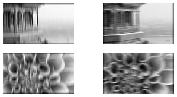

alt text

Các lớp Gộp (Pooling Layers)

Thực hành: Triển khai Pooling với PyTorch

# Tạo lớp Max Pooling với cửa sổ 2x2. Mặc định stride = kernel_size = 2
max_pool = nn.MaxPool2d(kernel_size=2)
output_max = max_pool(cropped_images)

# Tạo lớp Average Pooling với cửa sổ 2x2
avg_pool = nn.AvgPool2d(kernel_size=2)
output_avg = avg_pool(cropped_images)

fig = plt.figure(figsize=(8, 6))

# Ảnh gốc
ax1 = plt.subplot2grid((2, 3), (0, 0), rowspan=2, colspan=2)
ax1.imshow(cropped_images[0].permute(1, 2, 0))
ax1.axis('off')
ax1.set_title("Original image")

# Kết quả Max Pooling
ax2 = plt.subplot2grid((2, 3), (0, 2))
ax2.imshow(output_max[0].permute(1, 2, 0))
ax2.axis('off')
ax2.set_title("Max pooling")

# Kết quả Avg Pooling
ax3 = plt.subplot2grid((2, 3), (1, 2))
ax3.imshow(output_avg[0].permute(1, 2, 0))
ax3.axis('off')
ax3.set_title("Avg pooling")

plt.tight_layout()
plt.show()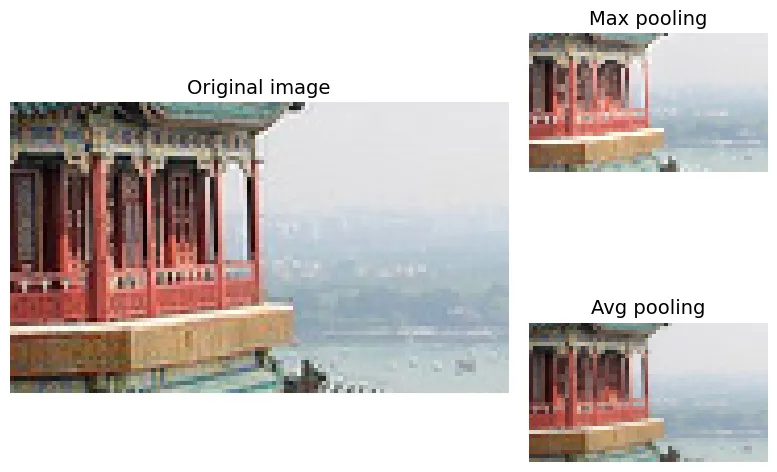

alt text

Depth-wise Pooling:

class DepthMaxPool2(torch.nn.Module):
    def __init__(self, kernel_size, stride=None, padding=0):
        super().__init__()
        self.kernel_size = kernel_size
        self.stride = stride if stride is not None else kernel_size
        self.padding = padding

    def forward(self, inputs):
        batch, channels, height, width = inputs.shape
        # Gộp chiều không gian lại để xử lý chiều kênh như chiều dài chuỗi
        Z = inputs.view(batch, channels, height * width)
        Z = Z.permute(0, 2, 1)  # Hoán đổi: [batch, spatial, channels]
        # Dùng MaxPool1d trên chiều channels
        Z = F.max_pool1d(Z, kernel_size=self.kernel_size, stride=self.stride,
                         padding=self.padding)
        Z = Z.permute(0, 2, 1)  # Hoán đổi ngược lại
        return Z.view(batch, -1, height, width)  # Phục hồi chiều không gian

Global Average Pooling (GAP):

global_avg_pool = nn.AvgPool2d(kernel_size=(70, 120))
output = global_avg_pool(cropped_images)

global_avg_pool = nn.AdaptiveAvgPool2d(output_size=1)
output = global_avg_pool(cropped_images)

output = cropped_images.mean(dim=(2, 3), keepdim=True)

Các kiến trúc CNN (CNN Architectures)

Giải quyết Fashion MNIST với CNN

Xây dựng mạng CNN: [Conv -> ReLU -> Pool] x 3 -> Flatten -> Dense.

from functools import partial

torch.manual_seed(42)

# Định nghĩa một lớp Conv2d mặc định với kernel 3x3 và padding="same"
DefaultConv2d = partial(nn.Conv2d, kernel_size=3, padding="same")

model = nn.Sequential(
    # Lớp 1: 64 filters, kernel 7x7 (lớn để bắt đặc trưng cơ bản), giảm kích thước bằng MaxPool
    DefaultConv2d(in_channels=1, out_channels=64, kernel_size=7), nn.ReLU(),
    nn.MaxPool2d(kernel_size=2),

    # Lớp 2: Tăng lên 128 filters
    DefaultConv2d(in_channels=64, out_channels=128), nn.ReLU(),
    DefaultConv2d(in_channels=128, out_channels=128), nn.ReLU(),
    nn.MaxPool2d(kernel_size=2),

    # Lớp 3: Tăng lên 256 filters
    DefaultConv2d(in_channels=128, out_channels=256), nn.ReLU(),
    DefaultConv2d(in_channels=256, out_channels=256), nn.ReLU(),
    nn.MaxPool2d(kernel_size=2),

    # Phần phân loại (Classifier)
    nn.Flatten(),
    nn.Linear(in_features=2304, out_features=128), nn.ReLU(),
    nn.Dropout(0.5), # Dropout để chống overfitting
    nn.Linear(in_features=128, out_features=64), nn.ReLU(),
    nn.Dropout(0.5),
    nn.Linear(in_features=64, out_features=10),
).to(device)

Các hàm huấn luyện:

import torchmetrics

def evaluate_tm(model, data_loader, metric):
    model.eval() # Chuyển sang chế độ đánh giá (tắt dropout, batchnorm update)
    metric.reset()
    with torch.no_grad(): # Không tính gradient để tiết kiệm bộ nhớ
        for X_batch, y_batch in data_loader:
            X_batch, y_batch = X_batch.to(device), y_batch.to(device)
            y_pred = model(X_batch)
            metric.update(y_pred, y_batch)
    return metric.compute()

def train(model, optimizer, loss_fn, metric, train_loader, valid_loader,
          n_epochs):
    history = {"train_losses": [], "train_metrics": [], "valid_metrics": []}
    for epoch in range(n_epochs):
        total_loss = 0.0
        metric.reset()
        model.train() # Chuyển sang chế độ huấn luyện
        for X_batch, y_batch in train_loader:
            X_batch, y_batch = X_batch.to(device), y_batch.to(device)
            y_pred = model(X_batch)
            loss = loss_fn(y_pred, y_batch)

            # Backpropagation
            optimizer.zero_grad()
            loss.backward()
            optimizer.step()

            total_loss += loss.item()
            metric.update(y_pred, y_batch)

        # Lưu lịch sử huấn luyện
        history["train_losses"].append(total_loss / len(train_loader))
        history["train_metrics"].append(metric.compute().item())
        history["valid_metrics"].append(
            evaluate_tm(model, valid_loader, metric).item())

        print(f"Epoch {epoch + 1}/{n_epochs}, "
              f"train loss: {history['train_losses'][-1]:.4f}, "
              f"train metric: {history['train_metrics'][-1]:.4f}, "
              f"valid metric: {history['valid_metrics'][-1]:.4f}")
    return history

Chuẩn bị dữ liệu:

import torchvision
import torchvision.transforms.v2 as T

# Chuỗi biến đổi: chuyển sang Image object -> chuyển sang Tensor float32 và scale về [0,1]
toTensor = T.Compose([T.ToImage(), T.ToDtype(torch.float32, scale=True)])

train_and_valid_data = torchvision.datasets.FashionMNIST(
    root="datasets", train=True, download=True, transform=toTensor)
test_data = torchvision.datasets.FashionMNIST(
    root="datasets", train=False, download=True, transform=toTensor)

torch.manual_seed(42)
train_data, valid_data = torch.utils.data.random_split(
    train_and_valid_data, [55_000, 5_000])

output:
    100%|██████████| 26.4M/26.4M [00:02<00:00, 11.9MB/s]
    100%|██████████| 29.5k/29.5k [00:00<00:00, 204kB/s]
    100%|██████████| 4.42M/4.42M [00:01<00:00, 3.82MB/s]
    100%|██████████| 5.15k/5.15k [00:00<00:00, 16.9MB/s]

from torch.utils.data import DataLoader

torch.manual_seed(42)
train_loader = DataLoader(train_data, batch_size=32, shuffle=True)
valid_loader = DataLoader(valid_data, batch_size=32)
test_loader = DataLoader(test_data, batch_size=32)

Huấn luyện:

n_epochs = 20
optimizer = torch.optim.AdamW(model.parameters())
xentropy = nn.CrossEntropyLoss()
accuracy = torchmetrics.Accuracy(task="multiclass", num_classes=10).to(device)

history = train(model, optimizer, xentropy, accuracy,
                train_loader, valid_loader, n_epochs)

output:
    Epoch 1/20, train loss: 0.7853, train metric: 0.7155, valid metric: 0.8344
    ...
    Epoch 20/20, train loss: 0.1771, train metric: 0.9395, valid metric: 0.9052

Kiến trúc Xception

Lớp Tích chập tách biệt (Separable Convolutional Layer)

Xception cải thiện hiệu suất bằng cách sử dụng Depthwise Separable Convolution, tách quá trình học thành hai bước: không gian (spatial) và độ sâu (depth/channel). Số lượng tham số giảm từ $C_{out} \cdot C_{in} \cdot k^2$ xuống còn $C_{in} \cdot k^2 + C_{in} \cdot C_{out}$ .

class SeparableConv2d(nn.Module):
    def __init__(self, in_channels, out_channels, kernel_size, stride=1,
                 padding=0):
        super().__init__()
        # Bước 1: Depthwise Conv (groups=in_channels nghĩa là mỗi kênh input có 1 filter riêng)
        self.depthwise_conv = nn.Conv2d(
            in_channels, in_channels, kernel_size, stride=stride,
            padding=padding, groups=in_channels)
        # Bước 2: Pointwise Conv (kernel 1x1 để trộn các kênh)
        self.pointwise_conv = nn.Conv2d(
            in_channels, out_channels, kernel_size=1, stride=1, padding=0)

    def forward(self, inputs):
        return self.pointwise_conv(self.depthwise_conv(inputs))

Triển khai ResNet-34 sử dụng PyTorch

Kiến trúc ResNet (Residual Network) giới thiệu các kết nối tắt (skip connections) $y = F(x) + x$ , giúp giải quyết vấn đề biến mất gradient khi huấn luyện mạng rất sâu.

class ResidualUnit(nn.Module):
    def __init__(self, in_channels, out_channels, stride=1):
        super().__init__()
        # Conv chuẩn với Batch Norm (bias=False vì BN đã có bias)
        DefaultConv2d = partial(
            nn.Conv2d, kernel_size=3, stride=1, padding=1, bias=False)

        self.main_layers = nn.Sequential(
            DefaultConv2d(in_channels, out_channels, stride=stride),
            nn.BatchNorm2d(out_channels),
            nn.ReLU(),
            DefaultConv2d(out_channels, out_channels),
            nn.BatchNorm2d(out_channels),
        )

        # Xử lý skip connection: Nếu stride > 1 hoặc số kênh thay đổi,
        # cần dùng conv 1x1 để khớp kích thước trước khi cộng.
        if stride > 1 or in_channels != out_channels:
            self.skip_connection = nn.Sequential(
                DefaultConv2d(in_channels, out_channels, kernel_size=1,
                              stride=stride, padding=0),
                nn.BatchNorm2d(out_channels),
            )
        else:
            self.skip_connection = nn.Identity()

    def forward(self, inputs):
        # F(x) + x, sau đó mới áp dụng ReLU
        return F.relu(self.main_layers(inputs) + self.skip_connection(inputs))

class ResNet34(nn.Module):
    def __init__(self):
        super().__init__()
        # Các lớp khởi đầu của ResNet
        layers = [
            nn.Conv2d(in_channels=3, out_channels=64, kernel_size=7, stride=2,
                      padding=3, bias=False),
            nn.BatchNorm2d(num_features=64),
            nn.ReLU(),
            nn.MaxPool2d(kernel_size=3, stride=2, padding=1),
        ]

        # Xây dựng các khối Residual
        prev_filters = 64
        # ResNet-34 cấu trúc: [3, 4, 6, 3] blocks cho các kênh [64, 128, 256, 512]
        for filters in [64] * 3 + [128] * 4 + [256] * 6 + [512] * 3:
            stride = 1 if filters == prev_filters else 2
            layers.append(ResidualUnit(prev_filters, filters, stride=stride))
            prev_filters = filters

        # Các lớp cuối cùng
        layers += [
            nn.AdaptiveAvgPool2d(output_size=1),
            nn.Flatten(),
            nn.LazyLinear(10), # LazyLinear tự động suy luận input features
        ]
        self.resnet = nn.Sequential(*layers)

    def forward(self, inputs):
        return self.resnet(inputs)

torch.manual_seed(42)
model = ResNet34().to(device)
# Thử nghiệm với một batch ngẫu nhiên
images = torch.randn(2, 3, 224, 224).to(device)
model(images).shape

output:
    torch.Size([2, 10])

Sử dụng các Mô hình Tiền huấn luyện (Pretrained Models) của TorchVision

Sử dụng ConvNeXt Base đã được huấn luyện trên ImageNet.

# Tải trọng số đã huấn luyện trên ImageNet
weights = torchvision.models.ConvNeXt_Base_Weights.IMAGENET1K_V1
model = torchvision.models.convnext_base(weights=weights).to(device)

output:
    Downloading: "https://download.pytorch.org/models/convnext_base-6075fbad.pth" to /root/.cache/torch/hub/checkpoints/convnext_base-6075fbad.pth
    100%|██████████| 338M/338M [00:03<00:00, 89.1MB/s]

# Kiểm tra thư mục cache nơi chứa các models
torch.hub.get_dir()

output:
    '/root/.cache/torch/hub'

# Liệt kê tất cả các mô hình có sẵn trong torchvision
torchvision.models.list_models()[:5] # Hiển thị 5 cái đầu

output:
    ['alexnet',
     'convnext_base',
     'convnext_large',
     'convnext_small',
     'convnext_tiny']

list(torchvision.models.get_model_weights("convnext_base"))

output:
    [ConvNeXt_Base_Weights.IMAGENET1K_V1]

transform = weights.transforms()
preprocessed_images = transform(sample_images_permuted)

# Dự đoán thử trên ảnh mẫu
model.eval()
with torch.no_grad():
    y_logits = model(preprocessed_images.to(device))

# Logits là giá trị thô đầu ra trước khi qua hàm Softmax
y_logits.shape

output:
    torch.Size([2, 1000])

y_pred = torch.argmax(y_logits, dim=1)
y_pred

output:
    tensor([698, 985], device='cuda:0')

# Lấy danh sách tên lớp (categories) từ metadata của weights
class_names = weights.meta["categories"]
[class_names[class_id] for class_id in y_pred]

output:
    ['palace', 'daisy']

# Top 3 dự đoán cao nhất
y_top3_logits, y_top3_class_ids = y_logits.topk(k=3, dim=1)
[[class_names[class_id] for class_id in top3] for top3 in y_top3_class_ids]

output:
    [['palace', 'monastery', 'lakeside'], ['daisy', 'pot', 'ant']]

# Xác suất dự đoán (Softmax)
y_top3_logits.softmax(dim=1)

output:
    tensor([[0.8617, 0.1186, 0.0198],
            [0.8110, 0.0962, 0.0928]], device='cuda:0')

Các mô hình Tiền huấn luyện cho Học chuyển giao (Transfer Learning)

Fine-tuning mô hình ConvNeXt trên bộ dữ liệu Flowers102.

# Tải dữ liệu Flowers102 và áp dụng transform tương ứng với mô hình ConvNeXt
DefaultFlowers102 = partial(torchvision.datasets.Flowers102, root="datasets",
                            transform=weights.transforms(), download=True)
train_set = DefaultFlowers102(split="train")
valid_set = DefaultFlowers102(split="val")
test_set = DefaultFlowers102(split="test")

output:
    100%|██████████| 345M/345M [00:24<00:00, 14.4MB/s]
    100%|██████████| 502/502 [00:00<00:00, 1.40MB/s]
    100%|██████████| 15.0k/15.0k [00:00<00:00, 32.4MB/s]

from torch.utils.data import DataLoader

train_loader = DataLoader(train_set, batch_size=32, shuffle=True)
valid_loader = DataLoader(valid_set, batch_size=32)
test_loader = DataLoader(test_set, batch_size=32)

# Danh sách tên các loài hoa
class_names = ['pink primrose', 'hard-leaved pocket orchid', 'canterbury bells', 'sweet pea', 'english marigold', 'tiger lily', 'moon orchid', 'bird of paradise', 'monkshood', 'globe thistle', 'snapdragon', "colt's foot", 'king protea', 'spear thistle', 'yellow iris', 'globe-flower', 'purple coneflower', 'peruvian lily', 'balloon flower', 'giant white arum lily', 'fire lily', 'pincushion flower', 'fritillary', 'red ginger', 'grape hyacinth', 'corn poppy', 'prince of wales feathers', 'stemless gentian', 'artichoke', 'sweet william', 'carnation', 'garden phlox', 'love in the mist', 'mexican aster', 'alpine sea holly', 'ruby-lipped cattleya', 'cape flower', 'great masterwort', 'siam tulip', 'lenten rose', 'barbeton daisy', 'daffodil', 'sword lily', 'poinsettia', 'bolero deep blue', 'wallflower', 'marigold', 'buttercup', 'oxeye daisy', 'common dandelion', 'petunia', 'wild pansy', 'primula', 'sunflower', 'pelargonium', 'bishop of llandaff', 'gaura', 'geranium', 'orange dahlia', 'pink-yellow dahlia?', 'cautleya spicata', 'japanese anemone', 'black-eyed susan', 'silverbush', 'californian poppy', 'osteospermum', 'spring crocus', 'bearded iris', 'windflower', 'tree poppy', 'gazania', 'azalea', 'water lily', 'rose', 'thorn apple', 'morning glory', 'passion flower', 'lotus', 'toad lily', 'anthurium', 'frangipani', 'clematis', 'hibiscus', 'columbine', 'desert-rose', 'tree mallow', 'magnolia', 'cyclamen', 'watercress', 'canna lily', 'hippeastrum', 'bee balm', 'ball moss', 'foxglove', 'bougainvillea', 'camellia', 'mallow', 'mexican petunia', 'bromelia', 'blanket flower', 'trumpet creeper', 'blackberry lily']

# Hiển thị một số ảnh mẫu từ tập huấn luyện
transform = torchvision.transforms.Compose([
    torchvision.transforms.ToTensor(),
    torchvision.transforms.CenterCrop(500),
])
flowers_to_display = DefaultFlowers102(split="train", transform=transform)
sample_flowers = sorted({y: img for img, y in flowers_to_display}.items())[:12]

plt.figure(figsize=(10, 6))
for class_id, image in sample_flowers:
    if class_id == 12: break
    plt.subplot(3, 4, class_id + 1)
    plot_image(image)
    plt.title(f"{class_id}: {class_names[class_id]}", fontsize=11)

plt.show()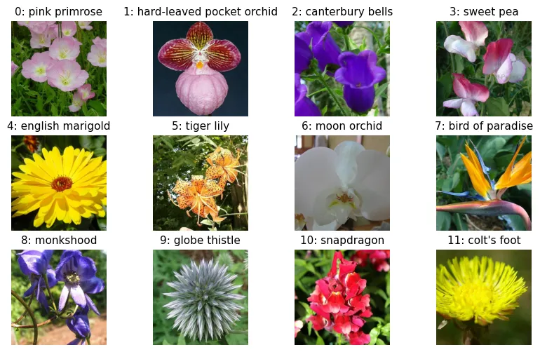

alt text

Thay thế lớp cuối cùng:

# Kiểm tra tên các lớp con trong model
[name for name, child in model.named_children()]

output:
    ['features', 'avgpool', 'classifier']

# Xem cấu trúc phần classifier
model.classifier

output:
    Sequential(
      (0): LayerNorm2d((1024,), eps=1e-06, elementwise_affine=True)
      (1): Flatten(start_dim=1, end_dim=-1)
      (2): Linear(in_features=1024, out_features=1000, bias=True)
    )

# Thay thế lớp Linear cuối cùng
n_classes = 102
model.classifier[2] = nn.Linear(1024, n_classes).to(device)

Chiến lược Freeze (Đóng băng) và Fine-tune (Tinh chỉnh):

# Đóng băng toàn bộ model
for param in model.parameters():
    param.requires_grad = False

# Mở đóng băng (unfreeze) phần classifier
for param in model.classifier.parameters():
    param.requires_grad = True

n_epochs = 5
optimizer = torch.optim.AdamW(model.parameters())
xentropy = nn.CrossEntropyLoss()
accuracy = torchmetrics.Accuracy(task="multiclass",
                                 num_classes=102).to(device)

# Huấn luyện (chỉ phần classifier)
history = train(model, optimizer, xentropy, accuracy,
                train_loader, valid_loader, n_epochs)

output:
    Epoch 1/5, train loss: 4.2828, train metric: 0.1422, valid metric: 0.6206
    ...
    Epoch 5/5, train loss: 0.9400, train metric: 0.9441, valid metric: 0.8667

# Mở đóng băng toàn bộ
for param in model.parameters():
    param.requires_grad = True

# Tiếp tục huấn luyện
history = train(model, optimizer, xentropy, accuracy,
                train_loader, valid_loader, n_epochs)

output:
    Epoch 1/5, train loss: 0.7673, train metric: 0.8265, valid metric: 0.8324
    ...
    Epoch 5/5, train loss: 0.0345, train metric: 0.9931, valid metric: 0.8814

Data Augmentation cho huấn luyện mạnh mẽ hơn:

import torchvision.transforms.v2 as T

transform = T.Compose([
    T.RandomHorizontalFlip(p=0.5),      # Lật ngang ngẫu nhiên
    T.RandomRotation(degrees=30),       # Xoay ngẫu nhiên
    T.RandomResizedCrop(size=(224, 224), scale=(0.8, 1.0)), # Cắt và thay đổi kích thước
    T.ColorJitter(brightness=0.2, contrast=0.2, saturation=0.2, hue=0.1), # Nhiễu màu
    T.ToImage(),
    T.ToDtype(torch.float32, scale=True),
    T.Normalize(mean=[0.485, 0.456, 0.406], std=[0.229, 0.224, 0.225]),
])

Phân loại và Định vị (Classification and Localization)

Định vị đối tượng là bài toán hồi quy (regression) dự đoán 4 tọa độ của bounding box.

class FlowerLocator(nn.Module):
    def __init__(self, base_model):
        super().__init__()
        self.base_model = base_model
        # Thêm nhánh định vị (localization head)
        self.localization_head = nn.Sequential(
            nn.Flatten(),
            nn.Linear(base_model.classifier[2].in_features, 4) # 4 tọa độ
        )

    def forward(self, X):
        # Trích xuất đặc trưng
        features = self.base_model.features(X)
        pool = self.base_model.avgpool(features)

        # Nhánh phân loại
        y_pred_logits = self.base_model.classifier(pool)

        # Nhánh định vị
        y_pred_bbox = self.localization_head(pool)
        return y_pred_logits, y_pred_bbox

torch.manual_seed(42)
locator_model = FlowerLocator(model).to(device)

preproc_images = torch.randn(2, 3, 224, 224)
y_pred_logits, y_pred_bbox = locator_model(preprocessed_images.to(device))

Xử lý Bounding Box:

import torchvision.tv_tensors

# Định nghĩa bounding box
bbox = torchvision.tv_tensors.BoundingBoxes(
    [[377, 199, 248, 262]],  # center x, center y, width, height
    format="CXCYWH",
    canvas_size=(500, 754)   # Kích thước ảnh gốc
)

# Thử biến đổi bbox
transform(bbox)

output:
    BoundingBoxes([[ 90,  91, 120, 154]], format=BoundingBoxFormat.CXCYWH, canvas_size=(224, 224), clamping_mode=soft)

torch.manual_seed(42)

first_image = torchvision.datasets.Flowers102(root="datasets", split="train")[0][0]

# Transform cả ảnh và label kèm bbox
preproc_image, preproc_target = transform(
    (first_image, {"label": 0, "bbox": bbox})
)
preproc_bbox = preproc_target["bbox"]

# Hàm vẽ bbox lên ảnh
def get_image_with_bbox(image, bbox, width=5, color="white"):
    # Chuyển đổi định dạng bbox sang XYXY để vẽ
    bbox_xyxy = torchvision.ops.box_convert(bbox, "cxcywh", "xyxy")
    return torchvision.utils.draw_bounding_boxes(
        image, bbox_xyxy, width=width, colors=color)

first_image_ts = T.ToImage()(first_image)
image_with_bbox = get_image_with_bbox(first_image_ts, bbox)
plot_image(image_with_bbox)
plt.show()

alt text

def denormalize(image, mean=[0.485, 0.456, 0.406], std=[0.229, 0.224, 0.225]):
    return (image * torch.tensor(std).view(-1, 1, 1)
            + torch.tensor(mean).view(-1, 1, 1))

image_with_bbox2 = get_image_with_bbox(
    denormalize(preproc_image), preproc_bbox, width=2, color="yellow")
plot_image(image_with_bbox2)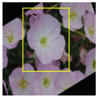

alt text

torch.manual_seed(42)

preproc_image2, preproc_target2 = transform(
    (image_with_bbox, {"label": 0, "bbox": bbox})
)
image_and_bbox3 = get_image_with_bbox(
    denormalize(preproc_image2), preproc_target2["bbox"], width=2, color="yellow")
plot_image(image_and_bbox3)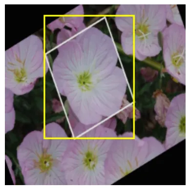

alt text

Tạo Dataset tùy chỉnh hỗ trợ BBox:

# Giả lập dữ liệu bbox cho 2 ảnh
bboxes = [
    torchvision.tv_tensors.BoundingBoxes(
        [[377, 199, 248, 262]],
        format="CXCYWH",
        canvas_size=(500, 754)
    ),
    torchvision.tv_tensors.BoundingBoxes(
        [[314, 248, 437, 445]],
        format="CXCYWH",
        canvas_size=(500, 624)
    )
]

class FlowersWithBBox(torch.utils.data.Dataset):
    def __init__(self, root, bboxes, transform=None, split="train"):
        self.image_dataset = torchvision.datasets.Flowers102(root=root,
                                                             split=split)
        self.bboxes = bboxes
        self.transform = transform

    def __len__(self):
        return len(self.bboxes)

    def __getitem__(self, index):
        raw_image, label = self.image_dataset[index]
        image = torchvision.tv_tensors.Image(raw_image)
        bbox = self.bboxes[index]
        # Áp dụng transform cho cả ảnh và bbox cùng lúc
        preproc_image, preproc_bbox = self.transform(image, bbox)
        return preproc_image, {"label": label, "bbox": preproc_bbox}

train_set_with_bboxes = FlowersWithBBox("datasets", bboxes, transform=transform)

train_loader_with_bboxes = DataLoader(train_set_with_bboxes, batch_size=2)
for images, label_and_bbox in train_loader_with_bboxes:
    label = label_and_bbox["label"]
    bbox = label_and_bbox["bbox"]
    # Tại đây, ta có thể tính loss cho cả classification (CrossEntropy) và localization (MSE hoặc IoU loss)

Phát hiện đối tượng (Object Detection)

Sử dụng YOLOv9 (You Only Look Once), một mô hình State-of-the-Art cho phát hiện đối tượng thời gian thực.

if IS_COLAB or IS_KAGGLE:
    %pip install -q ultralytics

output:
     [?25l    [90m━━━━━━━━━━━━━━━━━━━━━━━━━━━━━━━━━━━━━━━━ [0m  [32m0.0/1.2 MB [0m  [31m? [0m eta  [36m-:--:-- [0m
 [2K    [91m━━━━━━━━━━━━━━━━━━━━━━━━━━━━━━━━━━━━━━━ [0m [91m╸ [0m  [32m1.1/1.2 MB [0m  [31m44.4 MB/s [0m eta  [36m0:00:01 [0m
 [2K    [90m━━━━━━━━━━━━━━━━━━━━━━━━━━━━━━━━━━━━━━━━ [0m  [32m1.2/1.2 MB [0m  [31m30.1 MB/s [0m eta  [36m0:00:00 [0m
     [?25h

from ultralytics import YOLO

# Tải mô hình YOLOv9m (medium variant)
model = YOLO('yolov9m.pt')

# Dự đoán trên các ảnh mẫu từ internet
images = ["https://homl.info/soccer.jpg", "https://homl.info/traffic.jpg"]
results = model(images)

output:
    Downloading https://github.com/ultralytics/assets/releases/download/v8.3.0/yolov9m.pt to 'yolov9m.pt': 100% ━━━━━━━━━━━━ 39.1MB 75.2MB/s 0.5s
    
    0: 640x640 5 persons, 2 sports balls, 52.6ms
    1: 640x640 3 persons, 7 cars, 1 motorcycle, 11 trucks, 52.6ms
    Speed: 6.8ms preprocess, 52.6ms inference, 3.5ms postprocess per image at shape (1, 3, 640, 640)

# Chuyển kết quả sang pandas DataFrame để dễ xem
results[0].to_df()

output:
    (DataFrame hiển thị các box, class, confidence)

# Tóm tắt kết quả (số lượng đối tượng từng loại)
results[0].summary()[0]

output:
    {'name': 'sports ball',
     'class': 32,
     'confidence': 0.96212,
     'box': {'x1': 245.35858, 'y1': 286.03119, 'x2': 300.62524, 'y2': 343.57166}}

import PIL

# Lưu và hiển thị ảnh đã được đánh dấu (annotated)
results[0].save("my_annotated_soccer.jpg")
PIL.Image.open("my_annotated_soccer.jpg")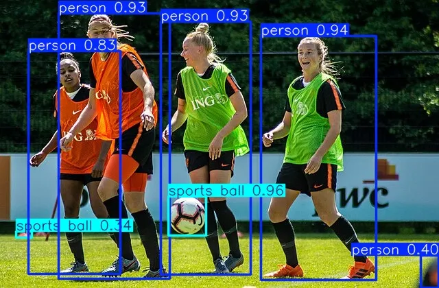

alt text

results[1].save("my_annotated_traffic.jpg")
PIL.Image.open("my_annotated_traffic.jpg")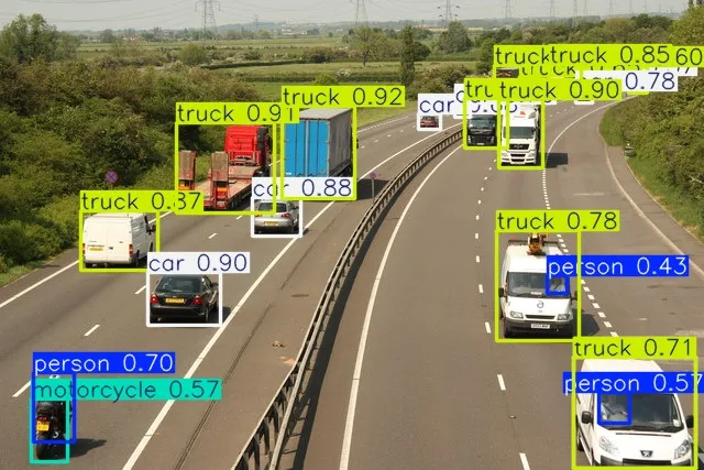

alt text

Theo dõi đối tượng (Object Tracking)

Object Tracking gán ID duy nhất cho các đối tượng qua các frame video.

my_video = "https://homl.info/cars.mp4"
# Sử dụng model.track để theo dõi
results = model.track(source=my_video, stream=True, save=True)

for frame_results in results:
    summary = frame_results.summary()
    # Lấy track_id của các đối tượng
    track_ids = [obj["track_id"] for obj in summary]
    print("Track ids:", track_ids)

output:
    Downloading https://homl.info/cars.mp4 to 'cars.mp4': 100% ━━━━━━━━━━━━ 14.7MB 108.6MB/s 0.1s
    video 1/1 (frame 1/243) /content/cars.mp4: 384x640 1 person, 8 cars, 1 bus, 1 truck, 92.2ms
    Track ids: [1, 2, 3, 4, 5, 6, 7, 8, 9, 10, 11]
    ...

Phân đoạn ngữ nghĩa (Semantic Segmentation)

Phân loại từng pixel trong ảnh. Sử dụng FCN-ResNet50.

from pathlib import Path
import urllib.request

def download_file(url, path):
    path = Path(path)
    if not path.is_file():
        path.parent.mkdir(parents=True, exist_ok=True)
        urllib.request.urlretrieve(url, path)

download_file("https://homl.info/soccer.jpg", "datasets/images/soccer.jpg")

from torchvision.models.segmentation import fcn_resnet50, FCN_ResNet50_Weights

weights = FCN_ResNet50_Weights.DEFAULT
model = fcn_resnet50(weights=weights)
model.eval()

img = PIL.Image.open("datasets/images/soccer.jpg")
transform = weights.transforms()
batch = transform(img).unsqueeze(0) # Thêm chiều batch

with torch.no_grad():
    # Model trả về dict, lấy key "out". Áp dụng softmax để ra xác suất từng lớp cho mỗi pixel
    masks = model(batch)["out"].softmax(dim=1)

# Lấy mask của lớp "person"
class_names = weights.meta["categories"]
name_to_id = {name: class_id for class_id, name in enumerate(class_names)}
mask = masks[0, name_to_id["person"]]

output:
    Downloading: "https://download.pytorch.org/models/fcn_resnet50_coco-1167a1af.pth" to /root/.cache/torch/hub/checkpoints/fcn_resnet50_coco-1167a1af.pth
    100%|██████████| 135M/135M [00:00<00:00, 213MB/s]

# Hiển thị mask
plt.imshow(mask, cmap="binary")
plt.axis('off')
plt.show()

alt text

# Phủ mask lên ảnh gốc để thấy vùng được chọn
masked_image = mask.unsqueeze(0) * denormalize(batch.squeeze(0))
plot_image(masked_image)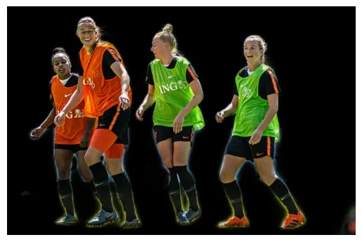

alt text

Phụ lục: Quan hệ giữa mAP và Precision/Recall

Mean Average Precision (mAP): Diện tích dưới đường cong Precision-Recall trung bình cho các mức IoU (Intersection over Union).

def maximum_precisions(precisions):
    # Tính đường bao phía trên (làm mượt đường cong)
    return np.flip(np.maximum.accumulate(np.flip(precisions)))

import numpy as np

recalls = np.linspace(0, 1, 11)
precisions = [0.91, 0.94, 0.96, 0.94, 0.95, 0.92, 0.80, 0.60, 0.45, 0.20, 0.10]
max_precisions = maximum_precisions(precisions)
mAP = max_precisions.mean()

plt.plot(recalls, precisions, "ro--", label="Precision")
plt.plot(recalls, max_precisions, "bo-", label="Max Precision")
plt.xlabel("Recall")
plt.ylabel("Precision")
plt.plot([0, 1], [mAP, mAP], "b:", linewidth=3, label="mAP")
plt.grid(True)
plt.axis([0, 1, 0, 1])
plt.legend(loc="lower center")
plt.show()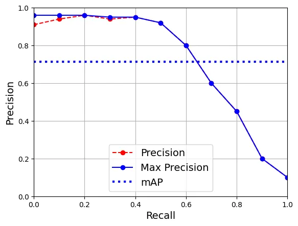

alt text

Thực hành 1: Xây dựng CNN độ chính xác cao cho MNIST

# Tải dữ liệu MNIST
toTensor = T.Compose([T.ToImage(), T.ToDtype(torch.float32, scale=True)])

train_and_valid_data = torchvision.datasets.MNIST(
    root="datasets", train=True, download=True, transform=toTensor)
test_data = torchvision.datasets.MNIST(
    root="datasets", train=False, download=True, transform=toTensor)

torch.manual_seed(42)
train_data, valid_data = torch.utils.data.random_split(
    train_and_valid_data, [55_000, 5_000])

output:
    100%|██████████| 9.91M/9.91M [00:00<00:00, 20.7MB/s]
    100%|██████████| 28.9k/28.9k [00:00<00:00, 491kB/s]
    100%|██████████| 1.65M/1.65M [00:00<00:00, 4.53MB/s]
    100%|██████████| 4.54k/4.54k [00:00<00:00, 7.55MB/s]

torch.manual_seed(42)
train_loader = DataLoader(train_data, batch_size=32, shuffle=True)
valid_loader = DataLoader(valid_data, batch_size=32)
test_loader = DataLoader(test_data, batch_size=32)

class MnistModel(nn.Module):
    def __init__(self):
        super().__init__()
        self.conv1 = nn.Conv2d(1, 32, kernel_size=3, padding=1)
        self.conv2 = nn.Conv2d(32, 64, kernel_size=3, padding=1)
        self.pool = nn.MaxPool2d(2)
        self.flatten = nn.Flatten()
        self.dropout1 = nn.Dropout(0.25)
        # Tính toán kích thước sau pool: 28x28 -> 14x14. 64 channels.
        self.fc1 = nn.Linear(1 * 14 * 14 * 64, 128)
        self.dropout2 = nn.Dropout(0.5)
        self.fc2 = nn.Linear(128, 10)

        # Khởi tạo trọng số Kaiming He (tốt cho ReLU)
        for m in self.modules():
            if isinstance(m, nn.Conv2d) or isinstance(m, nn.Linear):
                nn.init.kaiming_normal_(m.weight, nonlinearity="relu")
                if m.bias is not None:
                    nn.init.zeros_(m.bias)

    def forward(self, x):
        x = F.relu(self.conv1(x))
        x = F.relu(self.conv2(x))
        x = self.pool(x)
        x = self.flatten(x)
        x = self.dropout1(x)
        x = F.relu(self.fc1(x))
        x = self.dropout2(x)
        return self.fc2(x)

torch.manual_seed(42)
mnist_model = MnistModel().to(device)

n_epochs = 10
optimizer = torch.optim.AdamW(mnist_model.parameters())
xentropy = nn.CrossEntropyLoss()
accuracy = torchmetrics.Accuracy(task="multiclass",
                                 num_classes=10).to(device)

history = train(mnist_model, optimizer, xentropy, accuracy,
                train_loader, valid_loader, n_epochs)

output:
    Epoch 1/10, train loss: 0.2163, train metric: 0.9355, valid metric: 0.9828
    ...
    Epoch 10/10, train loss: 0.0262, train metric: 0.9915, valid metric: 0.9896

evaluate_tm(mnist_model, test_loader, accuracy)

output:
    tensor(0.9914, device='cuda:0')

Thực hành 2: Học chuyển giao cho phân loại ảnh lớn

from pathlib import Path
import urllib.request
import zipfile

def download_hymenoptera_dataset():
    data_dir = Path("datasets")
    url = "https://download.pytorch.org/tutorial/hymenoptera_data.zip"
    zip_path = data_dir / "hymenoptera_data.zip"
    data_dir.mkdir(parents=True, exist_ok=True)
    if not zip_path.exists():
        print("Downloading...",  end="")
        urllib.request.urlretrieve(url, zip_path)
        print(" Done.")
    unzipped_dir = data_dir / "hymenoptera_data"
    if not unzipped_dir.exists():
        print("Extracting...", end="")
        with zipfile.ZipFile(zip_path, "r") as zf:
            zf.extractall(data_dir)
        print(" Done.")
    return unzipped_dir

hymenoptera_dir = download_hymenoptera_dataset()

output:
    Downloading... Done.
    Extracting... Done.

import PIL
# Kiểm tra ảnh kiến và ong
PIL.Image.open(hymenoptera_dir / "train" / "ants" / "560966032_988f4d7bc4.jpg")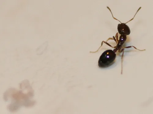

alt text

PIL.Image.open(hymenoptera_dir / "train" / "bees" / "760568592_45a52c847f.jpg")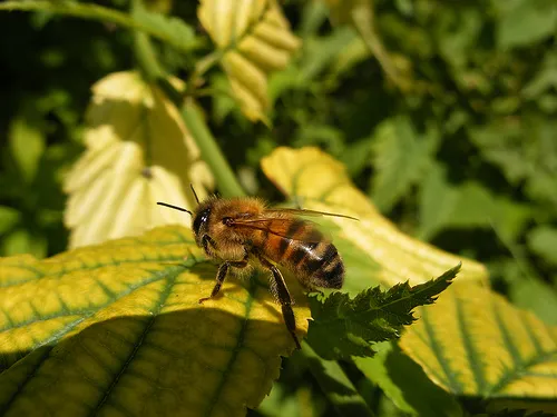

alt text

from torchvision.datasets import ImageFolder
import torchvision.transforms.v2 as T

# Transform cho tập train: có thêm augmentation (flip, crop)
train_transforms = T.Compose([
    T.RandomResizedCrop(224),
    T.RandomHorizontalFlip(),
    T.ToImage(),
    T.ToDtype(torch.float32, scale=True),
    T.Normalize([0.485, 0.456, 0.406], [0.229, 0.224, 0.225])
])

# Transform cho validation/test: chỉ resize và normalize
valid_test_transforms = T.Compose([
    T.Resize(232),
    T.CenterCrop(224),
    T.ToImage(),
    T.ToDtype(torch.float32, scale=True),
    T.Normalize([0.485, 0.456, 0.406], [0.229, 0.224, 0.225])
])

train_set = ImageFolder(hymenoptera_dir / "train", train_transforms)
valid_test_set = ImageFolder(hymenoptera_dir / "val", valid_test_transforms)

torch.manual_seed(42)
valid_set, test_set = torch.utils.data.random_split(valid_test_set, [0.5, 0.5])
class_names = train_set.classes

batch_size = 32
train_loader = DataLoader(train_set, batch_size=batch_size, shuffle=True)
valid_loader = DataLoader(valid_set, batch_size=batch_size)
test_loader = DataLoader(test_set, batch_size=batch_size)

Fine-tuning ConvNeXt cho 2 lớp (Ants vs Bees).

weights = torchvision.models.ConvNeXt_Base_Weights.IMAGENET1K_V1
model = torchvision.models.convnext_base(weights=weights).to(device)

# Thay thế classifier: output 2 lớp
model.classifier[2] = nn.Linear(1024, 2).to(device)

# Đóng băng feature extractor, chỉ train classifier
for param in model.parameters():
    param.requires_grad = False

for param in model.classifier.parameters():
    param.requires_grad = True

n_epochs = 5
optimizer = torch.optim.AdamW(model.parameters(), lr=1e-3)
xentropy = nn.CrossEntropyLoss()
accuracy = torchmetrics.Accuracy(task="multiclass", num_classes=2).to(device)

history = train(model, optimizer, xentropy, accuracy,
                train_loader, valid_loader, n_epochs)

output:
    Epoch 1/5, train loss: 0.4842, train metric: 0.8484, valid metric: 1.0000
    ...
    Epoch 5/5, train loss: 0.0545, train metric: 0.9918, valid metric: 1.0000

evaluate_tm(model, test_loader, accuracy)

output:
    tensor(0.9868, device='cuda:0')

Thực hành 3: Tinh chỉnh mô hình Phát hiện đối tượng

Bài tập này yêu cầu bạn làm theo hướng dẫn chi tiết tại PyTorch Object Detection Finetuning Tutorial. Đây là một quy trình phức tạp hơn bao gồm việc định nghĩa Dataset tùy chỉnh trả về bounding boxes, masks, và sử dụng Mask R-CNN.