[DL101] Chương 3: Huấn luyện Mạng Neron Sâu (Deep Neural Networks)
Các kỹ thuật huấn luyện mạng nơ-ron sâu: Vanishing Gradients, Optimizers, Regularization
Bài viết có tham khảo, sử dụng và sửa đổi tài nguyên từ kho lưu trữ handson-mlp, tuân thủ giấy phép Apache‑2.0. Chúng tôi chân thành cảm ơn tác giả Aurélien Géron (@aureliengeron) vì sự chia sẻ kiến thức tuyệt vời và những đóng góp quý giá cho cộng đồng.
Ở chương này, chúng ta sẽ cùng nhau giải quyết những thách thức cốt lõi trong việc huấn luyện Mạng Nơ-ron Sâu (Deep Neural Networks - DNNs).
Trong [DL101] Chương 2, chúng ta đã xây dựng nền móng với PyTorch. Tuy nhiên, lý thuyết và thực tiễn luôn có một khoảng cách lớn. Khi mạng nơ-ron trở nên “sâu” hơn (với hàng chục hoặc hàng trăm tầng ẩn), chúng ta không còn đơn thuần là xếp chồng các lớp tuyến tính và phi tuyến tính nữa. Chúng ta phải đối mặt với các hiện tượng toán học bất ổn định.
Tại sao việc huấn luyện DNN lại khó khăn?
- Gradient Instability (Bất ổn định Gradient): Trong quá trình lan truyền ngược, gradient là tích của các đạo hàm cục bộ (theo quy tắc chuỗi). Nếu các đạo hàm này nhỏ hơn 1, tích số sẽ tiến về 0 (Vanishing); nếu lớn hơn 1, tích số tiến về vô cùng (Exploding).
- Internal Covariate Shift: Sự phân phối của đầu vào tại các tầng ẩn thay đổi liên tục trong quá trình huấn luyện, buộc mạng phải liên tục thích nghi lại.
- Optimization Landscape: Bề mặt hàm mất mát của DNN không lồi (non-convex), chứa nhiều điểm yên ngựa (saddle points) và cực tiểu địa phương (local minima).
Chương này cung cấp các công cụ toán học và kỹ thuật thực nghiệm để kiểm soát các vấn đề trên.
Bạn có thể chạy trực tiếp các đoạn mã code tại: Google Colab.
Cài đặt môi trường
Để đảm bảo tính tái lập (reproducibility) trong nghiên cứu khoa học, việc kiểm soát phiên bản phần mềm là bắt buộc.
Kiểm tra phiên bản Python:
import sys

# Kiểm tra phiên bản Python phải >= 3.10
assert sys.version_info >= (3, 10)
Xác định môi trường thực thi (Runtime Environment):
IS_COLAB = "google.colab" in sys.modules
IS_KAGGLE = "kaggle_secrets" in sys.modules
Cài đặt thư viện bổ trợ TorchMetrics để tính toán các chỉ số đánh giá chuẩn xác:
if IS_COLAB:
    %pip install -q torchmetrics
output:
[?25l [90m━━━━━━━━━━━━━━━━━━━━━━━━━━━━━━━━━━━━━━━━ [0m [32m0.0/983.2 kB [0m [31m? [0m eta [36m-:--:-- [0m
[2K [91m━━━━━━━━━━━━━━━━━━━━━━━━━━━━━━━━━━━━━━━ [0m [91m╸ [0m [32m983.0/983.2 kB [0m [31m34.1 MB/s [0m eta [36m0:00:01 [0m
[2K [90m━━━━━━━━━━━━━━━━━━━━━━━━━━━━━━━━━━━━━━━━ [0m [32m983.2/983.2 kB [0m [31m19.2 MB/s [0m eta [36m0:00:00 [0m
[?25hKiểm tra phiên bản PyTorch:
from packaging.version import Version
import torch

# Kiểm tra phiên bản PyTorch
assert Version(torch.__version__) >= Version("2.6.0")
Deep Learning phụ thuộc nhiều vào khả năng tính toán song song của ma trận. Chúng ta ưu tiên sử dụng GPU (thông qua CUDA hoặc MPS).
if torch.cuda.is_available():
    device = "cuda"
elif torch.backends.mps.is_available():
    device = "mps"
else:
    device = "cpu"

device
output:
'cuda'Cảnh báo nếu không tìm thấy bộ tăng tốc phần cứng (GPU):
if device == "cpu":
    print("Mạng neron có thể chạy rất chậm nếu không có phần cứng tăng tốc.")
    if IS_COLAB:
        print("Vào Runtime > Change runtime type và chọn GPU hardware accelerator.")
    if IS_KAGGLE:
        print("Vào Settings > Accelerator và chọn GPU.")
Thiết lập cấu hình hiển thị biểu đồ:
import matplotlib.pyplot as plt

plt.rc('font', size=14)
plt.rc('axes', labelsize=14, titlesize=14)
plt.rc('legend', fontsize=14)
plt.rc('xtick', labelsize=10)
plt.rc('ytick', labelsize=10)
1. Vấn đề Biến mất và Bùng nổ Gradient (Vanishing/Exploding Gradients Problem)
Hãy xét một mạng nơ-ron đơn giản với tầng. Gradient tại tầng đầu tiên được tính bằng quy tắc chuỗi (Chain Rule): Trong đó phụ thuộc vào đạo hàm của hàm kích hoạt .
Nếu chúng ta sử dụng hàm Logistic Sigmoid: , đạo hàm của nó là . Giá trị cực đại của đạo hàm này chỉ là (tại ). Khi mạng sâu, tích của nhiều số nhỏ hơn sẽ tiến về 0 cực nhanh. Đây là hiện tượng Biến mất Gradient.
Ngược lại, nếu trọng số khởi tạo quá lớn, gradient có thể tăng theo cấp số nhân, dẫn đến Bùng nổ Gradient.
Đoạn mã sau minh họa tính chất “bão hòa” của hàm Sigmoid, nguyên nhân chính gây ra vấn đề này.
# extra code – đoạn mã này tạo ra Hình minh hoạ bên dưới

import numpy as np

def sigmoid(z):
    return 1 / (1 + np.exp(-z))

z = np.linspace(-5, 5, 200)

plt.plot([-5, 5], [0, 0], 'k-')
plt.plot([-5, 5], [1, 1], 'k--')
plt.plot([0, 0], [-0.2, 1.2], 'k-')
plt.plot([-5, 5], [-3/4, 7/4], 'g--')
plt.plot(z, sigmoid(z), "b-", linewidth=2,
         label=r"$\sigma(z) = \dfrac{1}{1+e^{-z}}$")
props = dict(facecolor='black', shrink=0.1)
plt.annotate('Saturating', xytext=(3.5, 0.7), xy=(5, 1), arrowprops=props,
             fontsize=14, ha="center")
plt.annotate('Saturating', xytext=(-3.5, 0.3), xy=(-5, 0), arrowprops=props,
             fontsize=14, ha="center")
plt.annotate('Linear', xytext=(2, 0.2), xy=(0, 0.5), arrowprops=props,
             fontsize=14, ha="center")
plt.grid(True)
plt.axis([-5, 5, -0.2, 1.2])
plt.xlabel("$z$")
plt.legend(loc="upper left", fontsize=16)

plt.show()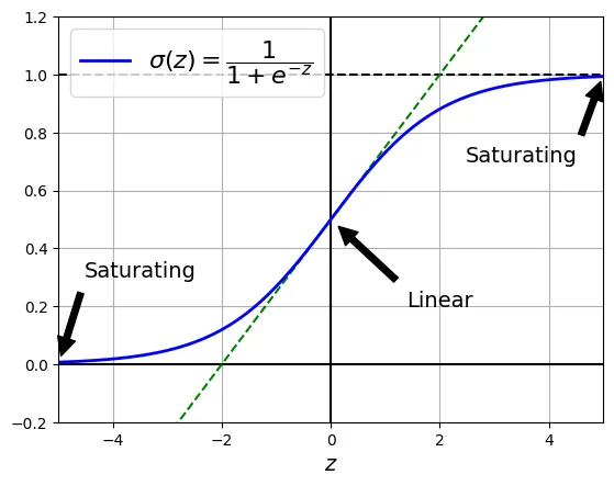
Khởi tạo Glorot và He (Glorot and He Initialization)
Để tín hiệu lan truyền ổn định, chúng ta cần phương sai (variance) của đầu ra bằng phương sai đầu vào tại mỗi tầng: . Glorot và Bengio (2010) đã chứng minh rằng với hàm kích hoạt tuyến tính (hoặc gần tuyến tính như Tanh đoạn giữa), trọng số nên được lấy mẫu từ phân phối có phương sai: Đây là Khởi tạo Xavier/Glorot.
Tuy nhiên, với hàm ReLU (chỉ dương), một nửa tín hiệu bị triệt tiêu (bằng 0). He et al. (2015) đã đề xuất tăng gấp đôi phương sai để bù đắp sự mất mát này: Đây là Khởi tạo He.
Bảng tóm tắt các chiến lược khởi tạo:
| Hàm kích hoạt | Phương pháp | Phương sai phân phối chuẩn |
|---|---|---|
| Logistic, Tanh, Softmax | Glorot (Xavier) | |
| ReLU, Leaky ReLU, ELU, GELU | He (Kaiming) | |
| SELU | LeCun |
import torch
import torch.nn as nn

layer = nn.Linear(40, 10)
# Khởi tạo He thủ công: Nhân trọng số với căn bậc hai của 6 (cho phân phối đều)
# hoặc căn bậc hai của 2 (cho phân phối chuẩn) chia cho n_in.
# Ở đây minh họa khái niệm nhân tỷ lệ.
layer.weight.data *= 6 ** 0.5  # Kaiming init (cho phân phối đều)
torch.zero_(layer.bias.data)   # Bias thường được khởi tạo bằng 0
output:
tensor([0., 0., 0., 0., 0., 0., 0., 0., 0., 0.])PyTorch cung cấp module torch.nn.init để thực hiện việc này một cách chuẩn tắc. Hàm kaiming_uniform_ thực hiện khởi tạo He với phân phối đều (Uniform Distribution).
layer = nn.Linear(40, 10)
# Sử dụng hàm kaiming_uniform_ có sẵn (tương đương He initialization)
nn.init.kaiming_uniform_(layer.weight)
nn.init.zeros_(layer.bias)
output:
Parameter containing:
tensor([0., 0., 0., 0., 0., 0., 0., 0., 0., 0.], requires_grad=True)Chúng ta có thể áp dụng chiến lược này cho toàn bộ mạng bằng phương thức .apply():
def use_he_init(module):
    # Chỉ áp dụng cho các lớp Linear (Kết nối đầy đủ)
    if isinstance(module, nn.Linear):
        nn.init.kaiming_uniform_(module.weight)
        nn.init.zeros_(module.bias)

model = nn.Sequential(nn.Linear(50, 40), nn.ReLU(), nn.Linear(40, 1), nn.ReLU())
model.apply(use_he_init) # Áp dụng hàm khởi tạo cho tất cả các module con
output:
Sequential(
(0): Linear(in_features=50, out_features=40, bias=True)
(1): ReLU()
(2): Linear(in_features=40, out_features=1, bias=True)
(3): ReLU()
)Đối với các hàm kích hoạt có tham số như LeakyReLU (), hệ số khởi tạo cần được điều chỉnh dựa trên độ dốc âm (negative slope).
model = nn.Sequential(nn.Linear(50, 40), nn.LeakyReLU(negative_slope=0.2))
model.apply(use_he_init)
output:
Sequential(
(0): Linear(in_features=50, out_features=40, bias=True)
(1): LeakyReLU(negative_slope=0.2)
)Các hàm kích hoạt tốt hơn (Better Activation Functions)
Hàm ReLU phổ biến vì tính toán nhanh, nhưng nó gặp vấn đề “Dying ReLU”: nếu , gradient bằng 0, nơ-ron ngừng học vĩnh viễn.
Leaky ReLU
Leaky ReLU khắc phục bằng cách cho phép một độ dốc nhỏ khi : Điều này đảm bảo dòng chảy gradient không bao giờ bị tắt hoàn toàn.
# extra code – đoạn mã này tạo ra Hình minh hoạ bên dưới

def leaky_relu(z, alpha):
    return np.maximum(alpha * z, z)

z = np.linspace(-5, 5, 200)
plt.plot(z, leaky_relu(z, 0.1), "b-", linewidth=2, label=r"$LeakyReLU(z) = max(\alpha z, z)$")
plt.plot([-5, 5], [0, 0], 'k-')
plt.plot([0, 0], [-1, 3.7], 'k-')
plt.grid(True)
props = dict(facecolor='black', shrink=0.1)
plt.annotate('Leak', xytext=(-3.5, 0.5), xy=(-5, -0.3), arrowprops=props,
             fontsize=14, ha="center")
plt.xlabel("$z$")
plt.axis([-5, 5, -1, 3.7])
plt.gca().set_aspect("equal")
plt.legend()

plt.show()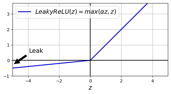
Khi sử dụng LeakyReLU, ta cần báo cho hàm khởi tạo Kaiming biết tham số a (tức là ) và chế độ nonlinearity='leaky_relu' để tính toán phương sai chính xác.
torch.manual_seed(42)
alpha = 0.2
model = nn.Sequential(nn.Linear(50, 40), nn.LeakyReLU(negative_slope=alpha))
# Chỉ định rõ 'leaky_relu' và tham số alpha cho hàm khởi tạo
nn.init.kaiming_uniform_(model[0].weight, a=alpha, nonlinearity="leaky_relu")
model(torch.rand(2, 50)).shape
output:
torch.Size([2, 40])ELU (Exponential Linear Unit)
ELU làm mượt phần âm bằng hàm mũ, giúp đẩy giá trị trung bình của đầu ra về gần 0 hơn, tăng tốc hội tụ.
torch.manual_seed(42)
model = nn.Sequential(nn.Linear(50, 40), nn.ELU())
# Khởi tạo He vẫn hoạt động tốt với ELU
nn.init.kaiming_uniform_(model[0].weight)
model(torch.rand(2, 50)).shape
output:
torch.Size([2, 40])SELU (Scaled ELU)
SELU là một phát kiến quan trọng (Klambauer et al., 2017). Nếu mạng nơ-ron thỏa mãn các điều kiện (dense layers, khởi tạo LeCun, input chuẩn hóa), mạng sẽ có tính chất tự chuẩn hóa (self-normalizing): đầu ra của mỗi lớp sẽ duy trì mean và std trong quá trình huấn luyện. Điều này giải quyết triệt để vấn đề biến mất/bùng nổ gradient.
# extra code – đoạn mã này tạo ra Hình minh hoạ bên dưới so sánh ELU và SELU

from scipy.special import erfc

# Các hằng số alpha và scale để đảm bảo tính tự chuẩn hóa (xem pt 14 trong bài báo gốc):
alpha_0_1 = -np.sqrt(2 / np.pi) / (erfc(1 / np.sqrt(2)) * np.exp(1 / 2) - 1)
scale_0_1 = (
    (1 - erfc(1 / np.sqrt(2)) * np.sqrt(np.e))
    * np.sqrt(2 * np.pi)
    * (
        2 * erfc(np.sqrt(2)) * np.e ** 2
        + np.pi * erfc(1 / np.sqrt(2)) ** 2 * np.e
        - 2 * (2 + np.pi) * erfc(1 / np.sqrt(2)) * np.sqrt(np.e)
        + np.pi
        + 2
    ) ** (-1 / 2)
)

def elu(z, alpha=1):
    return np.where(z < 0, alpha * (np.exp(z) - 1), z)

def selu(z, scale=scale_0_1, alpha=alpha_0_1):
    return scale * elu(z, alpha)

z = np.linspace(-5, 5, 200)
plt.plot(z, elu(z), "b-", linewidth=2, label=r"ELU$_\alpha(z) = \alpha (e^z - 1)$ if $z < 0$, else $z$")
plt.plot(z, selu(z), "r--", linewidth=2, label=r"SELU$(z) = 1.05 \, $ELU$_{1.67}(z)$")
plt.plot([-5, 5], [0, 0], 'k-')
plt.plot([-5, 5], [-1, -1], 'k:', linewidth=2)
plt.plot([-5, 5], [-1.758, -1.758], 'k:', linewidth=2)
plt.plot([0, 0], [-2.2, 3.2], 'k-')
plt.grid(True)
plt.axis([-5, 5, -2.2, 3.2])
plt.xlabel("$z$")
plt.gca().set_aspect("equal")
plt.legend()

plt.show()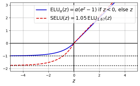
torch.manual_seed(42)
model = nn.Sequential(nn.Linear(50, 40), nn.SELU())
# Lưu ý: Khởi tạo trọng số phải dùng phương pháp LeCun (trong PyTorch gọi là 'fan_in')
# Tuy nhiên, kaiming_uniform_ cũng hoạt động khá ổn nếu cấu hình đúng
nn.init.kaiming_uniform_(model[0].weight)
model(torch.rand(2, 50)).shape
output:
torch.Size([2, 40])GELU, Swish, SwiGLU, Mish, và ReLU²
Các hàm kích hoạt hiện đại (thường dùng trong Transformer/LLM):
- GELU (Gaussian Error Linear Unit): .
- Swish (SiLU): .
- Mish: .
Chúng có đặc điểm chung là trơn (smooth) và không đơn điệu (non-monotonic) ở vùng âm, giúp tối ưu hóa gradient tốt hơn.
# extra code – tạo ra Hình minh hoạ bên dưới

def swish(z, beta=1):
    return z * sigmoid(beta * z)

def approx_gelu(z):
    return swish(z, beta=1.702)

def softplus(z):
    return np.log(1 + np.exp(z))

def mish(z):
    return z * np.tanh(softplus(z))

def relu_squared(z):
    return np.maximum(0, z)**2

z = np.linspace(-4, 2, 50)

beta = 0.6
plt.plot(z, approx_gelu(z), "b-", linewidth=2,
         label=r"GELU$(z) = z\,\Phi(z)$")
plt.plot(z, swish(z), "r--", linewidth=2,
         label=r"Swish$(z) = z\,\sigma(z)$")
plt.plot(z, swish(z, beta), "r:", linewidth=2,
         label=fr"Swish$_{{\beta={beta}}}(z)=z\,\sigma({beta}\,z)$")
plt.plot(z, mish(z), "k-.", linewidth=2,
         label=fr"Mish$(z) = z\,\tanh($softplus$(z))$")
plt.plot(z, relu_squared(z), "g.-", linewidth=1,
         label=fr"ReLU²$(z) = (\max(0, z))^2$")
plt.plot([-4, 2], [0, 0], 'k-')
plt.plot([0, 0], [-2.2, 3.2], 'k-')
plt.grid(True)
plt.axis([-4, 2, -1, 2])
plt.gca().set_aspect("equal")
plt.xlabel("$z$")
plt.legend(loc="upper left")

plt.show()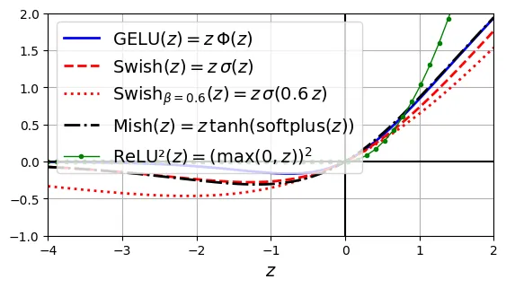
SwiGLU (Swish Gated Linear Unit): Biến thể sử dụng cổng (gating mechanism), cho hiệu suất rất cao trong các mô hình ngôn ngữ lớn (LLaMA).
class SwiGLU(nn.Module):
    def __init__(self, beta=1.0):
        super().__init__()
        self.beta = beta

    def forward(self, x):
        # Chia tensor đầu vào thành 2 phần
        z1, z2 = x.chunk(2, dim=-1)
        # Áp dụng cơ chế cổng (gate)
        param_swish = z1 * torch.sigmoid(self.beta * z1)
        return param_swish * z2

torch.manual_seed(42)
model = nn.Sequential(nn.Linear(50, 2 * 40), SwiGLU(beta=0.2))
nn.init.kaiming_uniform_(model[0].weight)
model(torch.rand(2, 50)).shape
output:
torch.Size([2, 40])ReLU² (Squared ReLU):
import torch.nn.functional as F

class ReLU2(nn.Module):
    def forward(self, x):
        return F.relu(x).square()

torch.manual_seed(42)
model = nn.Sequential(nn.Linear(50, 40), ReLU2())
nn.init.kaiming_uniform_(model[0].weight)
model(torch.rand(2, 50)).shape
output:
torch.Size([2, 40])Chuẩn hóa theo lô (Batch Normalization - BN)
Batch Normalization là kỹ thuật chèn thêm một lớp vào mô hình để chuẩn hóa các đầu vào của mỗi lớp ẩn. Thuật toán thực hiện 4 bước trên mỗi mini-batch :
- Tính trung bình batch: .
- Tính phương sai batch: .
- Chuẩn hóa: .
- Scale và Shift: . ( là tham số học được).
Kỹ thuật này giải quyết vấn đề Internal Covariate Shift (sự thay đổi phân phối đầu vào của các lớp ẩn), cho phép dùng tốc độ học lớn hơn và giảm sự phụ thuộc vào khởi tạo trọng số.
torch.manual_seed(42)

# Cách 1: BN sau hàm kích hoạt (Cấu hình cổ điển)
model = nn.Sequential(
    nn.Flatten(),
    nn.BatchNorm1d(1 * 28 * 28), # BN cho input
    nn.Linear(1 * 28 * 28, 300),
    nn.ReLU(),
    nn.BatchNorm1d(300),         # BN sau ReLU
    nn.Linear(300, 100),
    nn.ReLU(),
    nn.BatchNorm1d(100),
    nn.Linear(100, 10)
)
BN chứa các tham số có thể học được (weights , bias ) và các tham số thống kê chạy (running mean/var).
dict(model[1].named_parameters()).keys()output:
dict_keys(['weight', 'bias'])dict(model[1].named_buffers()).keys()output:
dict_keys(['running_mean', 'running_var', 'num_batches_tracked'])Cách 2 (Khuyến nghị): BN trước hàm kích hoạt. Khi đó, lớp Linear không cần bias (vì BN đã có đóng vai trò bias), giúp tiết kiệm tham số.
torch.manual_seed(42)

model = nn.Sequential(
    nn.Flatten(),
    nn.Linear(1 * 28 * 28, 300, bias=False), # Tắt bias
    nn.BatchNorm1d(300),
    nn.ReLU(),
    nn.Linear(300, 100, bias=False),
    nn.BatchNorm1d(100),
    nn.ReLU(),
    nn.Linear(100, 10)
)
Chuẩn hóa theo lớp (Layer Normalization - LN)
Khác với BN (chuẩn hóa dọc theo chiều batch), Layer Normalization chuẩn hóa dọc theo chiều đặc trưng (feature) cho từng mẫu dữ liệu riêng biệt. LN thường được dùng trong Mạng Nơ-ron Tái phát (RNN) và Transformer, nơi BN hoạt động kém hiệu quả do sự phụ thuộc vào batch size.
torch.manual_seed(42)

inputs = torch.randn(32, 3, 100, 200)  # batch gồm các ảnh RGB ngẫu nhiên
layer_norm = nn.LayerNorm([100, 200])
result = layer_norm(inputs)  # chuẩn hóa trên 2 chiều cuối (H, W)
Kiểm chứng thủ công công thức LN:
means = inputs.mean(dim=[2, 3], keepdim=True)
vars_ = inputs.var(dim=[2, 3], keepdim=True, unbiased=False)
stds = torch.sqrt(vars_ + layer_norm.eps)
result2 = layer_norm.weight * (inputs - means) / stds + layer_norm.bias
assert torch.allclose(result, result2)
# Chuẩn hóa trên cả 3 chiều cuối (C, H, W)
layer_norm = nn.LayerNorm([3, 100, 200])
result = layer_norm(inputs)Cắt Gradient (Gradient Clipping)
Đây là kỹ thuật giới hạn chuẩn (norm) của vector gradient không vượt quá một ngưỡng nào đó. Kỹ thuật này thường dùng để ngăn chặn Bùng nổ Gradient, đặc biệt trong RNN. Trong PyTorch, ta sử dụng nn.utils.clip_grad_norm_.
2. Tái sử dụng các tầng đã huấn luyện (Reusing Pretrained Layers)
Transfer Learning (Học chuyển giao) là kỹ thuật sử dụng kiến thức (trọng số) của một mô hình đã huấn luyện trên tập dữ liệu lớn (Source Task) để giải quyết một bài toán mới (Target Task). Điều này giúp:
- Giảm thời gian huấn luyện.
- Cần ít dữ liệu hơn cho bài toán mới.
- Cải thiện khả năng tổng quát hóa.
Transfer Learning với PyTorch
Chúng ta sẽ mô phỏng một kịch bản:
- Task A: Phân loại 8 loại quần áo (trừ Sandal và Shirt). Dữ liệu dồi dào.
- Task B: Phân loại nhị phân Sandal vs Shirt. Dữ liệu rất ít (200 mẫu).
from torch.utils.data import TensorDataset, DataLoader
from sklearn.datasets import fetch_openml

# Tải dữ liệu Fashion MNIST
fashion_mnist = fetch_openml(name="Fashion-MNIST", as_frame=False)
X = torch.FloatTensor(fashion_mnist.data.reshape(-1, 1, 28, 28) / 255.)
y = torch.from_numpy(fashion_mnist.target.astype(int))

# Tách dữ liệu thành tập A (không có lớp 0 và 2) và tập B (chỉ lớp 0 và 2)
in_B = (y == 0) | (y == 2)  # Pullover or T-shirt/top
X_A, y_A = X[~in_B], y[~in_B]
y_A = torch.maximum(y_A - 2, torch.tensor(0))  # Map lại nhãn: [1,3,4,5,6,7,8,9] => [0,..,7]
X_B, y_B = X[in_B], (y[in_B] == 2).to(dtype=torch.float32).view(-1, 1)

# Tạo Dataset
train_set_A = TensorDataset(X_A[:-7_000], y_A[:-7000])
valid_set_A = TensorDataset(X_A[-7_000:-5000], y_A[-7000:-5000])
test_set_A = TensorDataset(X_A[-5_000:], y_A[-5000:])
train_set_B = TensorDataset(X_B[:20], y_B[:20]) # Chỉ dùng 20 mẫu để train B
valid_set_B = TensorDataset(X_B[20:5000], y_B[20:5000])
test_set_B = TensorDataset(X_B[5_000:], y_B[5000:])

# Tạo DataLoader
train_loader_A = DataLoader(train_set_A, batch_size=32, shuffle=True)
valid_loader_A = DataLoader(valid_set_A, batch_size=32)
test_loader_A = DataLoader(test_set_A, batch_size=32)
train_loader_B = DataLoader(train_set_B, batch_size=32, shuffle=True)
valid_loader_B = DataLoader(valid_set_B, batch_size=32)
test_loader_B = DataLoader(test_set_B, batch_size=32)
Định nghĩa hàm huấn luyện và đánh giá chuẩn:
import torchmetrics

def evaluate_tm(model, data_loader, metric):
    model.eval()
    metric.reset()
    with torch.no_grad():
        for X_batch, y_batch in data_loader:
            X_batch, y_batch = X_batch.to(device), y_batch.to(device)
            y_pred = model(X_batch)
            metric.update(y_pred, y_batch)
    return metric.compute()

def train(model, optimizer, loss_fn, metric, train_loader, valid_loader,
          n_epochs):
    history = {"train_losses": [], "train_metrics": [], "valid_metrics": []}
    for epoch in range(n_epochs):
        total_loss = 0.0
        metric.reset()
        model.train()
        for X_batch, y_batch in train_loader:
            X_batch, y_batch = X_batch.to(device), y_batch.to(device)
            y_pred = model(X_batch)
            loss = loss_fn(y_pred, y_batch)
            total_loss += loss.item()
            loss.backward()
            # Bỏ comment dòng dưới để kích hoạt gradient clipping:
            #nn.utils.clip_grad_norm_(model.parameters(), max_norm=1.0)
            optimizer.step()
            optimizer.zero_grad()
            metric.update(y_pred, y_batch)
        history["train_losses"].append(total_loss / len(train_loader))
        history["train_metrics"].append(metric.compute().item())
        history["valid_metrics"].append(
            evaluate_tm(model, valid_loader, metric).item())
        print(f"Epoch {epoch + 1}/{n_epochs}, "
              f"train loss: {history['train_losses'][-1]:.4f}, "
              f"train metric: {history['train_metrics'][-1]:.4f}, "
              f"valid metric: {history['valid_metrics'][-1]:.4f}")
    return history
Huấn luyện Model A (8 lớp) - Giả sử đây là model đã được pre-train:
torch.manual_seed(42)

model_A = nn.Sequential(
    nn.Flatten(),
    nn.Linear(28 * 28, 100),
    nn.ReLU(),
    nn.Linear(100, 100),
    nn.ReLU(),
    nn.Linear(100, 100),
    nn.ReLU(),
    nn.Linear(100, 8)
)
model_A = model_A.to(device)
model_A.apply(use_he_init) # Khởi tạo He
output:
Sequential(
(0): Flatten(start_dim=1, end_dim=-1)
(1): Linear(in_features=784, out_features=100, bias=True)
(2): ReLU()
(3): Linear(in_features=100, out_features=100, bias=True)
(4): ReLU()
(5): Linear(in_features=100, out_features=100, bias=True)
(6): ReLU()
(7): Linear(in_features=100, out_features=8, bias=True)
)n_epochs = 20
optimizer = torch.optim.SGD(model_A.parameters(), lr=0.005)
xentropy = nn.CrossEntropyLoss()
accuracy = torchmetrics.Accuracy(task="multiclass", num_classes=8).to(device)
history_A = train(model_A, optimizer, xentropy, accuracy,
train_loader_A, valid_loader_A, n_epochs)output:
Epoch 1/20, train loss: 0.6363, train metric: 0.7845, valid metric: 0.8390
...
Epoch 20/20, train loss: 0.1691, train metric: 0.9394, valid metric: 0.9245Thử huấn luyện Model B từ đầu (không dùng transfer learning) với rất ít dữ liệu:
torch.manual_seed(9)

model_B = nn.Sequential(
    nn.Flatten(),
    nn.Linear(28 * 28, 100),
    nn.ReLU(),
    nn.Linear(100, 100),
    nn.ReLU(),
    nn.Linear(100, 100),
    nn.ReLU(),
    nn.Linear(100, 1)
).to(device)
model_B.apply(use_he_init)

n_epochs = 20
optimizer = torch.optim.SGD(model_B.parameters(), lr=0.005)
xentropy = nn.BCEWithLogitsLoss() # Binary Classification
accuracy = torchmetrics.Accuracy(task="binary").to(device)
history_B = train(model_B, optimizer, xentropy, accuracy,
                  train_loader_B, valid_loader_B, n_epochs)
output:
Epoch 1/20, train loss: 1.1117, train metric: 0.4000, valid metric: 0.5032
...
Epoch 20/20, train loss: 0.3815, train metric: 1.0000, valid metric: 0.8835evaluate_tm(model_B, test_loader_B, accuracy)output:
tensor(0.8860, device='cuda:0')Áp dụng Transfer Learning: Tái sử dụng các lớp của Model A cho Model B.
import copy

torch.manual_seed(43)
# Copy model A nhưng bỏ lớp cuối
reused_layers = copy.deepcopy(model_A[:-1])
model_B_on_A = nn.Sequential(
    *reused_layers,
    nn.Linear(100, 1)  # lớp output mới cho task B
).to(device)
Đóng băng (Freezing): Đặt requires_grad=False để trọng số của các lớp tái sử dụng không bị thay đổi trong những epoch đầu.
for layer in model_B_on_A[:-1]:
    for param in layer.parameters():
        param.requires_grad = False
n_epochs = 10
optimizer = torch.optim.SGD(model_B_on_A.parameters(), lr=0.005)
xentropy = nn.BCEWithLogitsLoss()
accuracy = torchmetrics.Accuracy(task="binary").to(device)
history_B = train(model_B_on_A, optimizer, xentropy, accuracy,
train_loader_B, valid_loader_B, n_epochs)output:
Epoch 1/10, train loss: 0.8847, train metric: 0.4000, valid metric: 0.4723
...
Epoch 10/10, train loss: 0.6148, train metric: 0.7500, valid metric: 0.7434Mở băng (Unfreezing) và Tinh chỉnh (Fine-tuning): Sau khi lớp cuối cùng đã học được kha khá, ta mở băng các lớp dưới để toàn bộ mạng cùng tinh chỉnh.
# Mở băng các lớp từ index 2 trở đi
for layer in model_B_on_A[2:]:
    for param in layer.parameters():
        param.requires_grad = True

n_epochs = 20
optimizer = torch.optim.SGD(model_B_on_A.parameters(), lr=0.005)
history_B = train(model_B_on_A, optimizer, xentropy, accuracy,
                  train_loader_B, valid_loader_B, n_epochs)
output:
Epoch 1/20, train loss: 0.6011, train metric: 0.7500, valid metric: 0.7709
...
Epoch 20/20, train loss: 0.3846, train metric: 0.9500, valid metric: 0.9307Kết quả: Độ chính xác trên tập kiểm tra tăng đáng kể nhờ Transfer Learning.
evaluate_tm(model_B_on_A, test_loader_B, accuracy)output:
tensor(0.9312, device='cuda:0')3. Các bộ tối ưu hóa nhanh hơn (Faster Optimizers)
Gradient Descent cơ bản (SGD) rất chậm. Chúng ta có các thuật toán tối ưu tốt hơn dựa trên hai ý tưởng chính: Momentum (quán tính) và Adaptive Learning Rate (tốc độ học thích ứng).
Hàm tiện ích để so sánh các optimizer:
# extra code – hàm tiện ích để kiểm tra optimizer trên Fashion MNIST

train_set = TensorDataset(X[:55_000], y[:55_000])
valid_set = TensorDataset(X[55_000:60_000], y[55_000:60_000])
test_set = TensorDataset(X[60_000:], y[60_000:])

def build_model(seed=42):
    torch.manual_seed(seed)
    model = nn.Sequential(
        nn.Flatten(),
        nn.Linear(28 * 28, 100),
        nn.ReLU(),
        nn.Linear(100, 100),
        nn.ReLU(),
        nn.Linear(100, 100),
        nn.ReLU(),
        nn.Linear(100, 10)
    ).to(device)
    model.apply(use_he_init)
    return model

def test_optimizer(model, optimizer, n_epochs=10, batch_size=32):
    train_loader = DataLoader(train_set, batch_size=32, shuffle=True)
    valid_loader = DataLoader(valid_set, batch_size=32)
    test_loader = DataLoader(test_set, batch_size=32)
    xentropy = nn.CrossEntropyLoss()
    accuracy = torchmetrics.Accuracy(task="multiclass", num_classes=10)
    history = train(model, optimizer, xentropy, accuracy.to(device),
                    train_loader, valid_loader, n_epochs)
    return history, evaluate_tm(model, test_loader, accuracy)
Stochastic Gradient Descent (SGD):
model = build_model()
optimizer = torch.optim.SGD(model.parameters(), lr=0.05)
history_sgd, acc_sgd = test_optimizer(model, optimizer)
output:
Epoch 1/10, train loss: 0.5710, train metric: 0.7930, valid metric: 0.8436
...
Epoch 10/10, train loss: 0.2622, train metric: 0.9016, valid metric: 0.8710Momentum Optimization
Mô phỏng quả bóng lăn xuống dốc, tích lũy vận tốc (momentum). Thường . Nó giúp vượt qua các điểm cực tiểu địa phương nông và tăng tốc độ trên bề mặt phẳng.
model = build_model()
optimizer = torch.optim.SGD(model.parameters(), momentum=0.9, lr=0.05)
history_momentum, acc_momentum = test_optimizer(model, optimizer)
output:
Epoch 1/10, train loss: 0.6026, train metric: 0.7829, valid metric: 0.7866
...
Epoch 10/10, train loss: 0.3676, train metric: 0.8689, valid metric: 0.8582Nesterov Accelerated Gradient (NAG)
Cải tiến Momentum bằng cách đo gradient tại vị trí “dự đoán” () thay vì vị trí hiện tại. Giống như việc “nhìn trước khi nhảy”.
model = build_model()
optimizer = torch.optim.SGD(model.parameters(),
                            momentum=0.9, nesterov=True, lr=0.05)
history_nesterov, acc_nesterov = test_optimizer(model, optimizer)
output:
Epoch 1/10, train loss: 0.5486, train metric: 0.8048, valid metric: 0.8118
...
Epoch 10/10, train loss: 0.3372, train metric: 0.8799, valid metric: 0.8566AdaGrad
Giảm tốc độ học cho các tham số có gradient lớn (thường xuyên cập nhật) và tăng cho tham số có gradient nhỏ (ít cập nhật). Tuy nhiên, tích lũy liên tục làm tốc độ học giảm về 0 quá sớm với DNN.
model = build_model()
optimizer = torch.optim.Adagrad(model.parameters(), lr=0.05)
history_adagrad, acc_adagrad = test_optimizer(model, optimizer)
output:
Epoch 1/10, train loss: 0.5605, train metric: 0.8155, valid metric: 0.8612
...
Epoch 10/10, train loss: 0.2511, train metric: 0.9060, valid metric: 0.8864RMSProp
Khắc phục AdaGrad bằng cách dùng trung bình di động lũy thừa (Exponential Moving Average) để chỉ quan tâm đến các gradient gần đây.
model = build_model()
optimizer = torch.optim.RMSprop(model.parameters(), alpha=0.9, lr=0.05)
history_rmsprop, acc_rmsprop = test_optimizer(model, optimizer)
output:
Epoch 1/10, train loss: 3.0856, train metric: 0.4135, valid metric: 0.4846
...
Epoch 10/10, train loss: 1.7721, train metric: 0.3072, valid metric: 0.2708Nhận xét: RMSProp với learning rate lớn (0.05) có thể không ổn định. Adam thường mạnh mẽ hơn.
Adam Optimization
Adam (Adaptive Moment Estimation) kết hợp Momentum và RMSProp: theo dõi cả trung bình gradient (moment bậc 1) và trung bình bình phương gradient (moment bậc 2).
model = build_model()
optimizer = torch.optim.Adam(model.parameters(), betas=(0.9, 0.999), lr=0.05)
history_adam, acc_adam = test_optimizer(model, optimizer)
output:
Epoch 1/10, train loss: 1.4496, train metric: 0.4273, valid metric: 0.4526
...
Epoch 10/10, train loss: 1.6109, train metric: 0.3166, valid metric: 0.2960Các biến thể của Adam:
- Adamax: Sử dụng chuẩn vô cực (infinity norm).
- Nadam: Adam kết hợp Nesterov.
- AdamW: Adam với Weight Decay được tách biệt (Decoupled Weight Decay), giúp chính quy hóa tốt hơn.
model = build_model()
optimizer = torch.optim.Adamax(model.parameters(), betas=(0.9, 0.999), lr=0.05)
history_adamax, acc_adamax = test_optimizer(model, optimizer)
output:
Epoch 1/10, train loss: 0.6799, train metric: 0.7774, valid metric: 0.7860
...
Epoch 10/10, train loss: 0.4032, train metric: 0.8580, valid metric: 0.8546model = build_model()
optimizer = torch.optim.NAdam(model.parameters(), betas=(0.9, 0.999), lr=0.05)
history_nadam, acc_nadam = test_optimizer(model, optimizer)output:
Epoch 1/10, train loss: 2.2631, train metric: 0.1478, valid metric: 0.1046
...
Epoch 10/10, train loss: 2.3088, train metric: 0.0985, valid metric: 0.1042model = build_model()
optimizer = torch.optim.AdamW(model.parameters(), betas=(0.9, 0.999),
weight_decay=1e-5, lr=0.05)
history_adamw, acc_adamw = test_optimizer(model, optimizer)output:
Epoch 1/10, train loss: 1.3913, train metric: 0.4717, valid metric: 0.3906
...
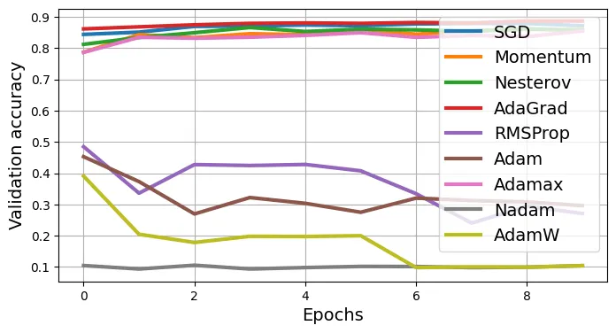
Epoch 10/10, train loss: 2.3120, train metric: 0.0975, valid metric: 0.1042So sánh trực quan:
# extra code – vẽ biểu đồ đường cong học tập của tất cả optimizer

for plot in ("train_losses", "valid_metrics"):
    plt.figure(figsize=(8, 4))
    opt_names = "SGD Momentum Nesterov AdaGrad RMSProp Adam Adamax Nadam AdamW"
    for history, opt_name in zip(
        (history_sgd, history_momentum, history_nesterov, history_adagrad,
         history_rmsprop, history_adam, history_adamax, history_nadam,
         history_adamw), opt_names.split()):
        plt.plot(history[plot], label=opt_name, linewidth=3)

    plt.grid()
    plt.xlabel("Epochs")
    plt.ylabel({"train_losses": "Training loss", "valid_metrics": "Validation accuracy"}[plot])
    plt.legend(loc="upper right")
    plt.show()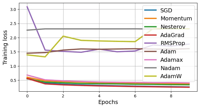
4. Lập lịch Tốc độ học (Learning Rate Scheduling)
Thay vì giữ LR cố định, việc giảm dần LR giúp mô hình hội tụ sâu hơn vào cực tiểu toàn cục.
Exponential Scheduling:
model = build_model()
optimizer = torch.optim.SGD(model.parameters(), lr=0.05)
# Giảm LR theo hàm mũ: nhân với 0.9 sau mỗi epoch
exp_scheduler = torch.optim.lr_scheduler.ExponentialLR(optimizer, gamma=0.9)
Cập nhật hàm train để hỗ trợ scheduler:
def train_with_scheduler(model, optimizer, loss_fn, metric, train_loader,
                         valid_loader, n_epochs, scheduler):
    history = {"train_losses": [], "train_metrics": [], "valid_metrics": []}
    for epoch in range(n_epochs):
        losses = []
        metric.reset()
        for X_batch, y_batch in train_loader:
            model.train()
            X_batch, y_batch = X_batch.to(device), y_batch.to(device)
            y_pred = model(X_batch)
            loss = loss_fn(y_pred, y_batch)
            losses.append(loss.item())
            loss.backward()
            optimizer.step()
            optimizer.zero_grad()
            metric.update(y_pred, y_batch)
        history["train_losses"].append(np.mean(losses))
        history["train_metrics"].append(metric.compute().item())
        val_metric = evaluate_tm(model, valid_loader, metric).item()
        history["valid_metrics"].append(val_metric)
        print(f"Epoch {epoch + 1}/{n_epochs}, "
              f"train loss: {history['train_losses'][-1]:.4f}, "
              f"train metric: {history['train_metrics'][-1]:.4f}, "
              f"valid metric: {history['valid_metrics'][-1]:.4f}")

        # Cập nhật scheduler
        if isinstance(scheduler, torch.optim.lr_scheduler.ReduceLROnPlateau):
            scheduler.step(val_metric)
        else:
            scheduler.step()
        print(f"Learning rate: {scheduler.get_last_lr()[0]:.5f}")
    return history

def test_scheduler(model, optimizer, scheduler, n_epochs=10, batch_size=32):
    train_loader = DataLoader(train_set, batch_size=32, shuffle=True)
    valid_loader = DataLoader(valid_set, batch_size=32)
    test_loader = DataLoader(test_set, batch_size=32)
    xentropy = nn.CrossEntropyLoss()
    metric = torchmetrics.Accuracy(task="multiclass", num_classes=10).to(device)
    history = train_with_scheduler(
        model, optimizer, xentropy, metric, train_loader, valid_loader,
        n_epochs, scheduler)
    return history, evaluate_tm(model, test_loader, metric)
history_exp, acc_exp = test_scheduler(model, optimizer, exp_scheduler)output:
Epoch 1/10, train loss: 0.5710, train metric: 0.7930, valid metric: 0.8436
Learning rate: 0.04500
...
Learning rate: 0.01743ReduceLROnPlateau: Giảm LR khi performance ngừng cải thiện (Performance Scheduling).
model = build_model()
optimizer = torch.optim.SGD(model.parameters(), lr=0.05)
# Giảm LR 10 lần nếu validation accuracy không tăng trong 2 epoch liên tiếp
perf_scheduler = torch.optim.lr_scheduler.ReduceLROnPlateau(
    optimizer, mode="max", patience=2, factor=0.1)
history_perf, acc_perf = test_scheduler(model, optimizer, perf_scheduler)output:
Epoch 1/10, train loss: 0.5710, train metric: 0.7930, valid metric: 0.8436
Learning rate: 0.05000
...
Learning rate: 0.050001Cycle Scheduling: Tăng LR từ thấp lên cao (warmup) rồi giảm xuống. Kỹ thuật này giúp mô hình vượt qua vùng phẳng ban đầu nhanh chóng và hội tụ siêu nhanh (super-convergence).
model = build_model()
optimizer = torch.optim.SGD(model.parameters(), lr=0.05)
warmup_scheduler = torch.optim.lr_scheduler.LinearLR(
    optimizer, start_factor=0.1, end_factor=1.0, total_iters=3)
# Hàm huấn luyện kết hợp warmup và scheduler chính
def train_with_warmup(model, optimizer, loss_fn, metric, train_loader,
valid_loader, n_epochs, warmup_scheduler, scheduler):
history = {"train_losses": [], "train_metrics": [], "valid_metrics": []}
for epoch in range(n_epochs):
# Bước warmup scheduler trước mỗi epoch
warmup_scheduler.step()
losses = []
metric.reset()
for X_batch, y_batch in train_loader:
model.train()
X_batch, y_batch = X_batch.to(device), y_batch.to(device)
y_pred = model(X_batch)
loss = loss_fn(y_pred, y_batch)
losses.append(loss.item())
loss.backward()
optimizer.step()
optimizer.zero_grad()
metric.update(y_pred, y_batch)
history["train_losses"].append(np.mean(losses))
history["train_metrics"].append(metric.compute().item())
val_metric = evaluate_tm(model, valid_loader, metric).item()
history["valid_metrics"].append(val_metric)
print(f"Epoch {epoch + 1}/{n_epochs}, "
f"train loss: {history['train_losses'][-1]:.4f}, "
f"train metric: {history['train_metrics'][-1]:.4f}, "
f"valid metric: {history['valid_metrics'][-1]:.4f}")
if epoch >= 3: # Sau khi warmup xong mới kích hoạt scheduler chính
scheduler.step(val_metric)
print(f"Learning rate: {scheduler.get_last_lr()[0]:.5f}")
return history
def test_warmup_scheduler(model, optimizer, warmup_scheduler, scheduler,
n_epochs=10, batch_size=32):
train_loader = DataLoader(train_set, batch_size=32, shuffle=True)
valid_loader = DataLoader(valid_set, batch_size=32)
test_loader = DataLoader(test_set, batch_size=32)
xentropy = nn.CrossEntropyLoss()
metric = torchmetrics.Accuracy(task="multiclass", num_classes=10).to(device)
history = train_with_warmup(
model, optimizer, xentropy, metric, train_loader, valid_loader,
n_epochs, warmup_scheduler, scheduler)
return history, evaluate_tm(model, test_loader, metric)perf_scheduler = torch.optim.lr_scheduler.ReduceLROnPlateau(
optimizer, mode="max", patience=2, factor=0.1)
test_warmup_scheduler(model, optimizer, warmup_scheduler, perf_scheduler,
n_epochs=10, batch_size=32)output:
Epoch 1/10, train loss: 0.6286, train metric: 0.7788, valid metric: 0.8356
Learning rate: 0.00500
...
Learning rate: 0.00500
(..., tensor(0.8653, device='cuda:0'))Hình minh họa các chiến lược điều chỉnh LR:
# Minh họa trực quan các hàm schedule khác: Cosine và Exponential
t = np.linspace(0, 20, 400)
eta_min = 0.001
eta_max = 0.05
t2 = 20
eta_cos_t = eta_min + 0.5 * (eta_max - eta_min) * (1 + np.cos(t / t2 * np.pi))
eta_exp_t = 0.9 ** t * eta_max

plt.figure(figsize=(8, 3))
plt.hlines([eta_min, eta_max], 0, 20, color="k", linestyle="dotted")
plt.plot(t, eta_cos_t, label="Cosine")
plt.plot(t, eta_exp_t, "--", label="Exponential")
plt.legend(loc="center right")
plt.text(10, eta_min + 0.0025, r"$\eta_\text{min}$")
plt.text(10, eta_max - 0.005, r"$\eta_\text{max}$")
plt.axis([0, 20, 0, eta_max * 1.05])
plt.grid(True)
plt.xlabel("Epoch")
plt.ylabel("Learning rate")
plt.show()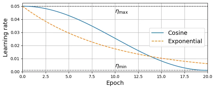
model = build_model()
optimizer = torch.optim.SGD(model.parameters(), lr=0.05)
cosine_repeat_scheduler = torch.optim.lr_scheduler.CosineAnnealingWarmRestarts(
    optimizer, T_0=2, T_mult=2, eta_min=0.001)

lrs = []
for epoch in range(62):
    lrs.append(cosine_repeat_scheduler.get_last_lr()[0])
    cosine_repeat_scheduler.step()

plt.figure(figsize=(8, 3))
plt.hlines([eta_min, eta_max], 0, 64, color="k", linestyle="dotted")
plt.plot(lrs, label="Cosine")
plt.text(30.5, eta_max - 0.005, r"$\eta_\text{max}$")
plt.text(58, eta_min + 0.003, r"$\eta_\text{min}$")
plt.axis([0, 62, 0, eta_max * 1.05])
plt.grid(True)
plt.xlabel("Epoch")
plt.ylabel("Learning rate")
plt.show()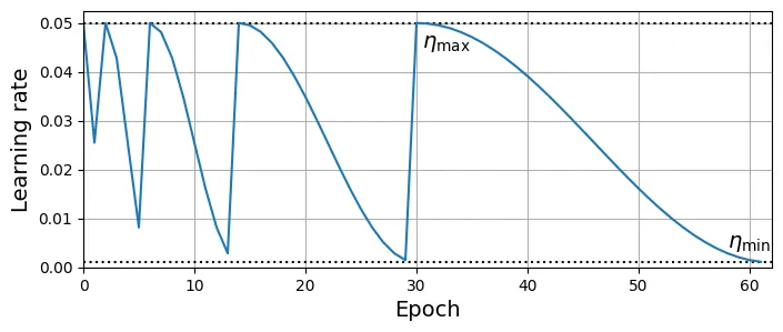
import re

DOCS_URL = "https://pytorch.org/docs/stable/generated/torch.optim.lr_scheduler"
for name in sorted(dir(torch.optim.lr_scheduler)):
    scheduler = getattr(torch.optim.lr_scheduler, name)
    if (not name.startswith("_") and isinstance(scheduler, type) and
        issubclass(scheduler, torch.optim.lr_scheduler.LRScheduler)):
            print(f"• {DOCS_URL}.{name}.html")
output:
• https://pytorch.org/docs/stable/generated/torch.optim.lr_scheduler.ChainedScheduler.html
...
• https://pytorch.org/docs/stable/generated/torch.optim.lr_scheduler.StepLR.html5. Tránh Quá Khớp Thông Qua Chính Quy Hóa (Regularization)
Chính quy hóa ℓ₁ và ℓ₂ (ℓ₁ and ℓ₂ regularization)
Thêm một số hạng phạt vào hàm mất mát để hạn chế độ lớn của trọng số:
- L2 (Weight Decay): . Ép trọng số nhỏ, giảm độ phức tạp mô hình.
- L1 (Lasso): . Ép trọng số về 0 (tạo mô hình thưa).
PyTorch tích hợp L2 qua tham số weight_decay.
model = build_model()
# weight_decay chính là hệ số lambda của L2 regularization
optimizer = torch.optim.SGD(model.parameters(), lr=0.05, weight_decay=1e-4)
history = test_optimizer(model, optimizer)
output:
Epoch 1/10, train loss: 0.5705, train metric: 0.7923, valid metric: 0.8528
...
Epoch 10/10, train loss: 0.2641, train metric: 0.9015, valid metric: 0.8666Cài đặt L2 thủ công (nếu cần linh hoạt hơn, ví dụ không phạt bias):
n_epochs = 3
train_loader = DataLoader(train_set, batch_size=32, shuffle=True)
loss_fn = nn.CrossEntropyLoss()

model = build_model()
optimizer = torch.optim.SGD(model.parameters(), lr=0.05)
params_to_regularize = [
    param for name, param in model.named_parameters()
    if not "bias" in name and not "bn" in name] # Loại trừ bias và batch norm

for epoch in range(n_epochs):
    total_loss = 0.0
    total_l2_loss = 0.0
    for X_batch, y_batch in train_loader:
        model.train()
        X_batch, y_batch = X_batch.to(device), y_batch.to(device)
        y_pred = model(X_batch)
        main_loss = loss_fn(y_pred, y_batch)
        # Tính L2 loss thủ công: tổng bình phương trọng số
        l2_loss = sum(param.pow(2.0).sum() for param in params_to_regularize)
        loss = main_loss + 1e-4 * l2_loss
        total_loss += loss.item()
        total_l2_loss += l2_loss.item()
        loss.backward()
        optimizer.step()
        optimizer.zero_grad()
    print(f"Epoch {epoch + 1}/{n_epochs}"
          f" – l2 loss: {total_l2_loss / len(train_loader):.3f}"
          f" – loss: {total_loss / len(train_loader):.3f}")
output:
Epoch 1/3 – l2 loss: 637.471 – loss: 0.634
Epoch 2/3 – l2 loss: 647.278 – loss: 0.467
Epoch 3/3 – l2 loss: 649.363 – loss: 0.427L1 Regularization (không hỗ trợ trực tiếp trong Optimizer, phải cài thủ công):
n_epochs = 3
train_loader = DataLoader(train_set, batch_size=32, shuffle=True)
loss_fn = nn.CrossEntropyLoss()

model = build_model()
optimizer = torch.optim.SGD(model.parameters(), lr=0.05)
params_to_regularize = [
    param for name, param in model.named_parameters()
    if not "bias" in name and not "bn" in name]
for epoch in range(n_epochs):
    total_loss = 0.0
    total_l1_loss = 0.0
    for X_batch, y_batch in train_loader:
        model.train()
        X_batch, y_batch = X_batch.to(device), y_batch.to(device)
        y_pred = model(X_batch)
        main_loss = loss_fn(y_pred, y_batch)
        # L1 loss: tổng trị tuyệt đối trọng số
        l1_loss = sum(param.abs().sum() for param in params_to_regularize)
        loss = main_loss + 1e-4 * l1_loss
        total_loss += loss.item()
        total_l1_loss += l1_loss.item()
        loss.backward()
        optimizer.step()
        optimizer.zero_grad()
    print(f"Epoch {epoch + 1}/{n_epochs}"
          f" – l1 loss: {total_l1_loss / len(train_loader):.3f}"
          f" – loss: {total_loss / len(train_loader):.3f}")
output:
Epoch 1/3 – l1 loss: 5703.592 – loss: 1.144
Epoch 2/3 – l1 loss: 5098.592 – loss: 0.919
Epoch 3/3 – l1 loss: 4552.979 – loss: 0.829Dropout
Dropout ngẫu nhiên “tắt” các nơ-ron với xác suất trong quá trình huấn luyện. Điều này buộc mạng phải học các đặc trưng mạnh mẽ hơn và hoạt động giống như một tổ hợp (ensemble) của nhiều mạng con.
torch.manual_seed(42)
model = nn.Sequential(
    nn.Flatten(),
    nn.Dropout(p=0.2), nn.Linear(28 * 28, 100), nn.ReLU(),
    nn.Dropout(p=0.2), nn.Linear(100, 100), nn.ReLU(),
    nn.Dropout(p=0.2), nn.Linear(100, 10)
).to(device)
model.apply(use_he_init)
optimizer = torch.optim.SGD(model.parameters(), lr=0.01, momentum=0.9)
history_dropout, acc_dropout = test_optimizer(model, optimizer, batch_size=32)
output:
Epoch 1/10, train loss: 0.6795, train metric: 0.7514, valid metric: 0.8384
...
Epoch 10/10, train loss: 0.3937, train metric: 0.8556, valid metric: 0.8738Monte-Carlo (MC) Dropout
Sử dụng Dropout ngay cả khi dự đoán (inference) để ước lượng độ không chắc chắn (uncertainty) của mô hình (theo lý thuyết Bayesian approximation).
# Bật Dropout thủ công (chuyển các lớp Dropout về chế độ train)
model.eval()
for module in model.modules():
    if isinstance(module, nn.Dropout):
        module.train()

# Lấy 3 ảnh mẫu
X_new = torch.FloatTensor(fashion_mnist.data[:3].reshape(3, 1, 28, 28) / 255)
X_new = X_new.to(device)

torch.manual_seed(42)
with torch.no_grad():
    # Lặp lại đầu vào 100 lần để dự đoán 100 lần khác nhau (do dropout)
    X_new_repeated = X_new.repeat_interleave(100, dim=0)
    y_logits_all = model(X_new_repeated).reshape(3, 100, 10)
    y_probas_all = torch.nn.functional.softmax(y_logits_all, dim=-1)
    # Lấy trung bình các dự đoán
y_probas = y_probas_all.mean(dim=1)y_probas.round(decimals=2)output:
tensor([[0.0000, 0.0000, 0.0000, 0.0000, 0.0000, 0.0000, 0.0000, 0.0100, 0.0000,
0.9900],
[0.9900, 0.0000, 0.0000, 0.0000, 0.0000, 0.0000, 0.0100, 0.0000, 0.0000,
0.0000],
[0.4100, 0.0400, 0.0400, 0.2300, 0.0400, 0.0000, 0.2300, 0.0000, 0.0100,
0.0000]], device='cuda:0')Độ lệch chuẩn cho thấy độ không chắc chắn:
y_std = y_probas_all.std(dim=1)
y_std.round(decimals=2)
output:
tensor([[0.0000, 0.0000, 0.0000, 0.0000, 0.0000, 0.0000, 0.0000, 0.0200, 0.0000,
0.0200],
[0.0200, 0.0000, 0.0000, 0.0000, 0.0000, 0.0000, 0.0200, 0.0000, 0.0000,
0.0000],
[0.1700, 0.0300, 0.0300, 0.1300, 0.0500, 0.0000, 0.0900, 0.0000, 0.0100,
0.0000]], device='cuda:0')class McDropout(nn.Dropout):
def forward(self, input):
# Luôn bật dropout ngay cả khi model.eval() được gọi
return F.dropout(input, self.p, training=True)def mean_prediction(model, X, n_repeats):
X_new_repeated = X_new.repeat_interleave(n_repeats, dim=0)
y_logits = model(X_new_repeated)
y_logits_all = y_logits.reshape(X.shape[0], n_repeats, *y_logits.shape[1:])
y_probas_all = torch.nn.functional.softmax(y_logits_all, dim=-1)
return y_probas_all.mean(dim=1)with torch.no_grad():
y_mean_pred = mean_prediction(model, X_new, 100)
y_mean_pred.round(decimals=2)output:
tensor([[0.0000, 0.0000, 0.0000, 0.0000, 0.0000, 0.0000, 0.0000, 0.0200, 0.0000,
0.9800],
[0.9800, 0.0000, 0.0000, 0.0000, 0.0000, 0.0000, 0.0200, 0.0000, 0.0000,
0.0000],
[0.4000, 0.0500, 0.0400, 0.2400, 0.0400, 0.0000, 0.2200, 0.0000, 0.0100,
0.0000]], device='cuda:0')Max-Norm Regularization
Giới hạn chuẩn của vector trọng số đi vào mỗi nơ-ron: .
def apply_max_norm(model, max_norm=2, epsilon=1e-8, dim=1):
    with torch.no_grad():
        for name, param in model.named_parameters():
            if 'bias' not in name:
                actual_norm = param.norm(p=2, dim=dim, keepdim=True)
                target_norm = torch.clamp(actual_norm, 0, max_norm)
param *= target_norm / (epsilon + actual_norm)torch.manual_seed(42)
n_epochs = 3
train_loader = DataLoader(train_set, batch_size=32, shuffle=True)
loss_fn = nn.CrossEntropyLoss()
model = build_model()
optimizer = torch.optim.SGD(model.parameters(), lr=0.05)
for epoch in range(n_epochs):
total_loss = 0.0
for X_batch, y_batch in train_loader:
model.train()
X_batch, y_batch = X_batch.to(device), y_batch.to(device)
y_pred = model(X_batch)
loss = loss_fn(y_pred, y_batch)
total_loss += loss.item()
loss.backward()
optimizer.step()
optimizer.zero_grad()
# Áp dụng Max-Norm sau mỗi bước cập nhật
apply_max_norm(model)
print(f"Epoch {epoch + 1}/{n_epochs}"
f" – loss: {total_loss / len(train_loader):.3f}")output:
Epoch 1/3 – loss: 0.571
Epoch 2/3 – loss: 0.402
Epoch 3/3 – loss: 0.361Bài thực hành: Học sâu trên CIFAR10
Bài tập: Huấn luyện mạng nơ-ron sâu trên bộ dữ liệu CIFAR10 (ảnh màu 32x32, 10 lớp).
Bước 1: Tải dữ liệu
import torchvision
import torchvision.transforms.v2 as T

# Chuyển ảnh sang Tensor và scale giá trị về [0, 1]
toTensor = T.Compose([T.ToImage(), T.ToDtype(torch.float32, scale=True)])
train_and_valid_set = torchvision.datasets.CIFAR10(
    root="datasets", train=True, download=True, transform=toTensor)
test_set = torchvision.datasets.CIFAR10(
    root="datasets", train=False, download=True, transform=toTensor)
output:
100%|██████████| 170M/170M [00:03<00:00, 43.9MB/s]torch.manual_seed(42)
train_set, valid_set = torch.utils.data.random_split(
train_and_valid_set, [45_000, 5_000])batch_size = 128
train_loader = DataLoader(train_set, batch_size=batch_size)
valid_loader = DataLoader(valid_set, batch_size=batch_size)
test_loader = DataLoader(test_set, batch_size=batch_size)Bước 2: Xây dựng mô hình
Xây dựng DNN 20 tầng ẩn, 100 nơ-ron mỗi tầng, sử dụng SiLU (Swish) và khởi tạo He.
def use_he_init(module):
    if isinstance(module, nn.Linear):
        nn.init.kaiming_uniform_(module.weight)
        nn.init.zeros_(module.bias)
def build_deep_model(n_hidden, n_neurons, n_inputs, n_outputs):
# Tầng đầu vào
layers = [nn.Flatten(), nn.Linear(n_inputs, n_neurons), nn.SiLU()]
# Các tầng ẩn lặp lại
for _ in range(n_hidden - 1):
layers += [nn.Linear(n_neurons, n_neurons), nn.SiLU()]
# Tầng đầu ra
layers += [nn.Linear(n_neurons, n_outputs)]
model = torch.nn.Sequential(*layers)
model.apply(use_he_init)
return modeltorch.manual_seed(42)
model = build_deep_model(
n_hidden=20, n_neurons=100, n_inputs=3 * 32 * 32, n_outputs=10
).to(device)Bước 3: Huấn luyện với NAdam và Early Stopping
import time

def train_with_early_stopping(model, optimizer, loss_fn, metric, train_loader,
                              valid_loader, n_epochs, patience=10,
                              checkpoint_path=None, scheduler=None):
    checkpoint_path = checkpoint_path or "my_checkpoint.pt"
    history = {"train_losses": [], "train_metrics": [], "valid_metrics": []}
    best_metric = 0.0
    patience_counter = 0
    for epoch in range(n_epochs):
        total_loss = 0.0
        metric.reset()
        model.train()
        t0 = time.time()
        for X_batch, y_batch in train_loader:
            X_batch, y_batch = X_batch.to(device), y_batch.to(device)
            y_pred = model(X_batch)
            loss = loss_fn(y_pred, y_batch)
            total_loss += loss.item()
            loss.backward()
            optimizer.step()
            optimizer.zero_grad()
            metric.update(y_pred, y_batch)

        train_metric = metric.compute().item()
        valid_metric = evaluate_tm(model, valid_loader, metric).item()

        # Logic Early Stopping: Lưu model tốt nhất
        if valid_metric > best_metric:
            torch.save(model.state_dict(), checkpoint_path)
            best_metric = valid_metric
            best = " (best)"
            patience_counter = 0
        else:
            patience_counter += 1
            best = ""

        t1 = time.time()
        history["train_losses"].append(total_loss / len(train_loader))
        history["train_metrics"].append(train_metric)
        history["valid_metrics"].append(valid_metric)
        print(f"Epoch {epoch + 1}/{n_epochs}, "
              f"train loss: {history['train_losses'][-1]:.4f}, "
              f"train metric: {history['train_metrics'][-1]:.4f}, "
              f"valid metric: {history['valid_metrics'][-1]:.4f}{best}"
              f" in {t1 - t0:.1f}s"
        )
        if scheduler is not None:
            scheduler.step()
        if patience_counter >= patience:
            print("Early stopping!")
            break

    # Tải lại trạng thái tốt nhất của model
    model.load_state_dict(torch.load(checkpoint_path))
    return history
optimizer = torch.optim.NAdam(model.parameters(), lr=2e-3)
criterion = nn.CrossEntropyLoss()
accuracy = torchmetrics.Accuracy(task="multiclass", num_classes=10).to(device)n_epochs = 100
history = train_with_early_stopping(model, optimizer, criterion, accuracy,
train_loader, valid_loader, n_epochs)output:
Epoch 1/100, train loss: 2.1743, train metric: 0.1644, valid metric: 0.1786 (best) in 12.0s
...
Epoch 25/100, train loss: 1.6192, train metric: 0.4069, valid metric: 0.3650 in 12.1s
Early stopping!Nhận xét: Model rất sâu (20 tầng) mà không có BN rất khó học, accuracy thấp (~40%).
Bước 4: Thêm Batch Normalization
def build_deep_model_with_batch_norm(n_hidden, n_neurons, n_inputs, n_outputs):
    # Thêm BN sau mỗi tầng Linear, trước activation
    layers = [nn.Flatten(), nn.Linear(n_inputs, n_neurons),
              nn.BatchNorm1d(n_neurons), nn.SiLU()]
    for _ in range(n_hidden - 1):
        layers += [nn.Linear(n_neurons, n_neurons),
                   nn.BatchNorm1d(n_neurons), nn.SiLU()]

    layers += [nn.Linear(n_neurons, n_outputs)]
    model = torch.nn.Sequential(*layers)
    model.apply(use_he_init)
return modeltorch.manual_seed(42)
model = build_deep_model_with_batch_norm(
n_hidden=20, n_neurons=100, n_inputs=3 * 32 * 32, n_outputs=10
).to(device)optimizer = torch.optim.NAdam(model.parameters(), lr=2e-3)
criterion = nn.CrossEntropyLoss()
accuracy = torchmetrics.Accuracy(task="multiclass", num_classes=10).to(device)n_epochs = 100
history = train_with_early_stopping(model, optimizer, criterion, accuracy,
train_loader, valid_loader, n_epochs)output:
Epoch 1/100, train loss: 1.9239, train metric: 0.2956, valid metric: 0.3274 (best) in 13.8s
...
Epoch 16/100, train loss: 0.9253, train metric: 0.6765, valid metric: 0.3646 in 13.5s
Early stopping!Bước 5: Tự chuẩn hóa với SELU
class Standardize(nn.Module):
    def __init__(self, sample):
        super().__init__()
        flat = torch.flatten(sample, start_dim=1)
        mean = flat.mean(dim=0, keepdim=True)
        std = flat.std(dim=0, keepdim=True)
        self.register_buffer("mean", mean)
        self.register_buffer("std", std)

    def forward(self, x):
        return (x - self.mean) / self.std
# Tính toán mean và std trên toàn bộ tập train
all_images = torch.stack([img for img, _ in train_set])
standardize = Standardize(all_images)def use_lecun_init(module):
if isinstance(module, nn.Linear):
# LeCun init tương đương kaiming_normal_ với mode='fan_in' và nonlinearity='linear'
nn.init.kaiming_normal_(module.weight, mode="fan_in",
nonlinearity="linear")
nn.init.zeros_(module.bias)def build_deep_model_with_selu(n_hidden, n_neurons, n_inputs, n_outputs):
layers = [nn.Flatten(), standardize,
nn.Linear(n_inputs, n_neurons), nn.SELU()]
for _ in range(n_hidden - 1):
layers += [nn.Linear(n_neurons, n_neurons), nn.SELU()]
layers += [nn.Linear(n_neurons, n_outputs)]
model = torch.nn.Sequential(*layers)
model.apply(use_lecun_init)
return modeltorch.manual_seed(42)
model = build_deep_model_with_selu(
n_hidden=20, n_neurons=100, n_inputs=3 * 32 * 32, n_outputs=10
).to(device)optimizer = torch.optim.SGD(model.parameters(), lr=1e-3)
criterion = nn.CrossEntropyLoss()
accuracy = torchmetrics.Accuracy(task="multiclass", num_classes=10).to(device)n_epochs = 100
history = train_with_early_stopping(model, optimizer, criterion, accuracy,
train_loader, valid_loader, n_epochs)output:
Epoch 1/100, train loss: 2.0557, train metric: 0.2615, valid metric: 0.3162 (best) in 11.9s
...
Epoch 39/100, train loss: 1.1467, train metric: 0.6034, valid metric: 0.4524 in 11.6s
Early stopping!Bước 6: Alpha Dropout và MC Dropout
def build_deep_model_with_alpha_dropout(n_hidden, n_neurons, n_inputs,
                                        n_outputs, dropout_rate):
    layers = [nn.Flatten(), standardize,
              nn.Linear(n_inputs, n_neurons), nn.SELU(),
              nn.AlphaDropout(dropout_rate)] # AlphaDropout thay vì Dropout thường
    for _ in range(n_hidden - 1):
        layers += [nn.Linear(n_neurons, n_neurons), nn.SELU(),
                   nn.AlphaDropout(dropout_rate)]

    layers += [nn.Linear(n_neurons, n_outputs)]
    model = torch.nn.Sequential(*layers)
    model.apply(use_lecun_init)
return modeltorch.manual_seed(42)
model = build_deep_model_with_alpha_dropout(
n_hidden=20, n_neurons=100, n_inputs=3 * 32 * 32, n_outputs=10,
dropout_rate=0.1
).to(device)optimizer = torch.optim.NAdam(model.parameters(), lr=1e-3)
criterion = nn.CrossEntropyLoss()
accuracy = torchmetrics.Accuracy(task="multiclass", num_classes=10).to(device)n_epochs = 100
history = train_with_early_stopping(model, optimizer, criterion, accuracy,
train_loader, valid_loader, n_epochs)output:
Epoch 1/100, train loss: 2.1558, train metric: 0.1955, valid metric: 0.1844 (best) in 12.8s
...
Epoch 57/100, train loss: 1.3930, train metric: 0.5175, valid metric: 0.4408 in 12.8s
Early stopping!Bước 7: 1Cycle Scheduling
torch.manual_seed(42)
model = build_deep_model_with_alpha_dropout(
    n_hidden=20, n_neurons=100, n_inputs=3 * 32 * 32, n_outputs=10,
    dropout_rate=0.1
).to(device)n_epochs = 60
optimizer = torch.optim.NAdam(model.parameters(), lr=1e-3)
# OneCycleLR điều chỉnh LR tăng lên rồi giảm xuống trong suốt quá trình train
scheduler = torch.optim.lr_scheduler.OneCycleLR(
optimizer, epochs=n_epochs, steps_per_epoch=len(train_loader), max_lr=1e-2)
criterion = nn.CrossEntropyLoss()
accuracy = torchmetrics.Accuracy(task="multiclass", num_classes=10).to(device)history = train_with_early_stopping(model, optimizer, criterion, accuracy,
train_loader, valid_loader, n_epochs,
patience=20, scheduler=scheduler)output:
Epoch 1/60, train loss: 2.2694, train metric: 0.1694, valid metric: 0.2430 (best) in 13.1s
...
Epoch 60/60, train loss: 1.2397, train metric: 0.5661, valid metric: 0.4564 in 12.7s