[DL101] Chương 2: Xây dựng Mạng Nơ-ron với PyTorch

Bài viết có tham khảo, sử dụng và sửa đổi tài nguyên từ kho lưu trữ handson-mlp, tuân thủ giấy phép Apache‑2.0. Chúng tôi chân thành cảm ơn tác giả Aurélien Géron (@aureliengeron) vì sự chia sẻ kiến thức tuyệt vời và những đóng góp quý giá cho cộng đồng.

Trong chương này, chúng ta sẽ đi sâu vào PyTorch, một trong những nền tảng (framework) tính toán khoa học và Học sâu (Deep Learning) mạnh mẽ nhất hiện nay.

Về mặt kỹ thuật, PyTorch không chỉ là một thư viện Deep Learning mà còn là một thư viện tính toán tensor (tensor computation library) với khả năng tăng tốc phần cứng mạnh mẽ. Điểm khác biệt cơ bản về triết lý thiết kế của PyTorch so với các thư viện thế hệ cũ (như TensorFlow 1.x) nằm ở Biểu đồ tính toán động (Dynamic Computational Graph - Define-by-Run). Điều này cho phép cấu trúc mạng nơ-ron có thể thay đổi ngay trong thời gian thực thi (runtime), mang lại sự linh hoạt tối đa cho việc nghiên cứu và gỡ lỗi.

Chương này được cấu trúc để đưa bạn từ những viên gạch nền tảng của Đại số tuyến tính trên Tensor, qua cơ chế Autograd (tự động vi phân), đến việc xây dựng các kiến trúc phức tạp như Wide & Deep và Convolutional Neural Networks (CNN).

Bạn có thể chạy trực tiếp các đoạn mã code tại: Google Colab.

1. Thiết lập môi trường (Setup)

Dự án này yêu cầu Python 3.10 trở lên để tận dụng các tính năng mới nhất của ngôn ngữ, đồng thời đảm bảo tương thích với các “wheels” được biên dịch sẵn của PyTorch:

import sys

# Kiểm tra xem phiên bản Python hiện tại có lớn hơn hoặc bằng 3.10 hay không
assert sys.version_info >= (3, 10)

Chúng ta cũng cần Scikit-Learn phiên bản 1.6.1 trở lên:

from packaging.version import Version
import sklearn

# Đảm bảo Scikit-Learn là phiên bản mới
assert Version(sklearn.__version__) >= Version("1.6.1")

Đoạn mã dưới đây giúp xác định môi trường thực thi (Runtime Environment). Việc này quan trọng vì trên Google Colab hay Kaggle, chúng ta thường được cấp phát GPU miễn phí, và cần cài đặt các thư viện bổ trợ khác nhau.

IS_COLAB = "google.colab" in sys.modules
IS_KAGGLE = "kaggle_secrets" in sys.modules

Nếu đang sử dụng Colab, chúng ta cần cài đặt thêm:

• optuna: Một khung làm việc (framework) tối ưu hóa siêu tham số (Hyperparameter Optimization) sử dụng thuật toán Tree-structured Parzen Estimator (TPE).
• torchmetrics: Thư viện chuẩn hóa các phép đo đánh giá mô hình (metrics) trên PyTorch.

if IS_COLAB:
    %pip install -q optuna torchmetrics

Thành phần cốt lõi là PyTorch. Chúng ta cần phiên bản tối thiểu là 2.6.0 để sử dụng các tính năng mới như torch.compile (tối ưu hóa đồ thị tĩnh):

import torch

# Kiểm tra phiên bản PyTorch
assert Version(torch.__version__) >= Version("2.6.0")

Cuối cùng, thiết lập cấu hình cho thư viện trực quan hóa matplotlib. Việc hiển thị rõ ràng các biểu đồ (như learning curves) là rất quan trọng để chẩn đoán hiện tượng quá khớp (overfitting) hoặc chưa khớp (underfitting).

import matplotlib.pyplot as plt

# Thiết lập kích thước font chữ mặc định cho các thành phần biểu đồ
plt.rc('font', size=14)
plt.rc('axes', labelsize=14, titlesize=14)
plt.rc('legend', fontsize=14)
plt.rc('xtick', labelsize=10)
plt.rc('ytick', labelsize=10)

2. Các nền tảng cơ bản của PyTorch (PyTorch Fundamentals)

PyTorch được xây dựng xoay quanh cấu trúc dữ liệu Tensor. Trong toán học và vật lý, Tensor là một đối tượng hình học ánh xạ các vector và covector sang một số vô hướng. Trong Khoa học Máy tính, chúng ta đơn giản hóa Tensor như một mảng đa chiều (generalized $n$-dimensional array).

2.1. PyTorch Tensors

Tensor tương tự như ndarray trong NumPy nhưng có hai đặc điểm vượt trội:

1. Hỗ trợ GPU: Có thể di chuyển sang bộ nhớ của Card đồ họa để tính toán song song.
2. Hỗ trợ Autograd: Lưu trữ lịch sử các phép toán để tính đạo hàm tự động.

Dưới đây là một Tensor hạng 2 (Rank-2 Tensor), tương đương với một Ma trận trong Đại số tuyến tính:

import torch

# Tạo một tensor 2 chiều (ma trận) từ một list
X = torch.tensor([[1.0, 4.0, 7.0], [2.0, 3.0, 6.0]])
X

output:
    tensor([[1., 4., 7.],
            [2., 3., 6.]])

# Kiểm tra kích thước (shape) của tensor: (hàng, cột)
X.shape

output:
    torch.Size([2, 3])

Kiểu dữ liệu (dtype) quyết định độ chính xác của tính toán. Trong Deep Learning, float32 (độ chính xác đơn) thường được ưu tiên hơn float64 (độ chính xác kép) để tiết kiệm bộ nhớ và tăng tốc độ, dù chấp nhận sai số làm tròn nhỏ.

# Kiểm tra kiểu dữ liệu (data type) của các phần tử trong tensor
X.dtype

output:
    torch.float32

Thao tác chỉ mục (indexing) và cắt lát (slicing) tuân theo quy ước của Python/NumPy:

# Truy cập phần tử ở hàng 0, cột 1
X[0, 1]

output:
    tensor(4.)

# Lấy tất cả các hàng, chỉ lấy cột 1
X[:, 1]

output:
    tensor([4., 3.])

PyTorch hỗ trợ Broadcasting (cơ chế lan truyền). Khi thực hiện phép toán giữa tensor và một số vô hướng (scalar), số vô hướng đó được “lan truyền” để khớp kích thước với tensor. Về mặt toán học, phép toán 10 * (X + 1.0) thực hiện: $Y_{ij} = 10 \cdot (X_{ij} + 1)$ với mọi $i, j$.

# Phép cộng và nhân theo từng phần tử (broadcasting)
10 * (X + 1.0)

output:
    tensor([[20., 50., 80.],
            [30., 40., 70.]])

# Tính hàm mũ (exponential) cho từng phần tử
X.exp()

output:
    tensor([[   2.7183,   54.5981, 1096.6332],
            [   7.3891,   20.0855,  403.4288]])

Các phép toán giảm chiều (Reduction operations) như mean hay max tổng hợp thông tin của tensor.

# Tính giá trị trung bình của toàn bộ tensor
X.mean()

output:
    tensor(3.8333)

# Tìm giá trị lớn nhất dọc theo trục 0 (trục dọc - so sánh các hàng với nhau)
X.max(dim=0)

output:
    torch.return_types.max(
    values=tensor([2., 4., 7.]),
    indices=tensor([1, 0, 0]))

Phép nhân ma trận (Matrix Multiplication): Đây là phép toán nền tảng của mạng nơ-ron. Cho ma trận $A$ kích thước $(m \times n)$ và $B$ kích thước $(n \times p)$, tích $C = A \times B$ có kích thước $(m \times p)$, với phần tử $C_{ij} = \sum_{k=1}^n A_{ik} B_{kj}$. Trong code dưới đây, X @ X.T thực hiện nhân $X$ với ma trận chuyển vị của nó ($X^T$).

# Nhân ma trận X với ma trận chuyển vị của nó (X.T)
X @ X.T

output:
    tensor([[66., 56.],
            [56., 49.]])

Khả năng tương tác (Interoperability) với NumPy:

import numpy as np

# Chuyển đổi tensor sang numpy array
X.numpy()

output:
    array([[1., 4., 7.],
           [2., 3., 6.]], dtype=float32)

Lưu ý quan trọng: NumPy mặc định sử dụng float64, trong khi PyTorch (và GPU) tối ưu cho float32. Sự chuyển đổi ngầm định có thể gây tăng gấp đôi lượng bộ nhớ tiêu thụ không cần thiết.

# Tạo tensor từ numpy array.
# Lưu ý: Mặc định numpy dùng float64, pyTorch dùng float32.
torch.tensor(np.array([[1., 4., 7.], [2., 3., 6.]]))

output:
    tensor([[1., 4., 7.],
            [2., 3., 6.]], dtype=torch.float64)

# Chỉ định kiểu dữ liệu float32 khi tạo tensor
torch.tensor(np.array([[1., 4., 7.], [2., 3., 6.]]), dtype=torch.float32)

output:
    tensor([[1., 4., 7.],
            [2., 3., 6.]])

# Một cách khác để tạo FloatTensor trực tiếp
torch.FloatTensor(np.array([[1., 4., 7.], [2., 3., 6]]))

output:
    tensor([[1., 4., 7.],
            [2., 3., 6.]])

Cơ chế chia sẻ bộ nhớ (Memory Sharing): Hàm torch.from_numpy() tạo ra một Tensor đóng vai trò là “view” (khung nhìn) lên vùng nhớ của NumPy array. Điều này giúp tránh sao chép dữ liệu (Zero-copy), nhưng đồng nghĩa thay đổi ở một bên sẽ ảnh hưởng bên còn lại.

# code bổ sung: minh họa torch.from_numpy()
X2_np = np.array([[1., 4., 7.], [2., 3., 6]])
X2 = torch.from_numpy(X2_np)  # X2_np và X2 chia sẻ cùng bộ nhớ
X2_np[0, 1] = 88  # Thay đổi trên numpy array
X2  # Giá trị trên tensor cũng thay đổi theo

output:
    tensor([[ 1., 88.,  7.],
            [ 2.,  3.,  6.]], dtype=torch.float64)

# Gán giá trị mới cho cột 1 của tensor X
X[:, 1] = -99
X

output:
    tensor([[  1., -99.,   7.],
            [  2., -99.,   6.]])

Trong PyTorch, các hàm có hậu tố _ (underscore) biểu thị In-place Operations (phép toán tại chỗ). Chúng sửa đổi dữ liệu trực tiếp trên vùng nhớ hiện tại thay vì cấp phát vùng nhớ mới cho kết quả.

# Áp dụng hàm ReLU (Rectified Linear Unit) tại chỗ: thay các giá trị âm bằng 0
X.relu_()
X

output:
    tensor([[1., 0., 7.],
            [2., 0., 6.]])

Để thuận tiện cho người dùng NumPy chuyển sang, PyTorch duy trì sự tương đồng lớn về API:

# code bổ sung: liệt kê các hàm xuất hiện ở cả NumPy và PyTorch
functions = lambda mod: set(f for f in dir(mod) if callable(getattr(mod, f)))
", ".join(sorted(functions(torch) & functions(np)))

output:
    '__getattr__, abs, absolute, acos, acosh, add, all, allclose, amax, amin, angle, any, arange, arccos, arccosh, arcsin, arcsinh, arctan, arctan2, arctanh, argmax, argmin, argsort, argwhere, asarray, asin, asinh, atan, atan2, atanh, atleast_1d, atleast_2d, atleast_3d, bincount, bitwise_and, bitwise_left_shift, bitwise_not, bitwise_or, bitwise_right_shift, bitwise_xor, broadcast_shapes, broadcast_to, can_cast, ceil, clip, column_stack, concat, concatenate, conj, copysign, corrcoef, cos, cosh, count_nonzero, cov, cross, cumprod, cumsum, deg2rad, diag, diagflat, diagonal, diff, divide, dot, dsplit, dstack, dtype, einsum, empty, empty_like, equal, exp, exp2, expm1, eye, finfo, fix, flip, fliplr, flipud, float_power, floor, floor_divide, fmax, fmin, fmod, frexp, from_dlpack, frombuffer, full, full_like, gcd, gradient, greater, greater_equal, heaviside, histogram, histogramdd, hsplit, hstack, hypot, i0, iinfo, imag, inner, isclose, isfinite, isin, isinf, isnan, isneginf, isposinf, isreal, kron, lcm, ldexp, less, less_equal, linspace, load, log, log10, log1p, log2, logaddexp, logaddexp2, logical_and, logical_not, logical_or, logical_xor, logspace, matmul, max, maximum, mean, median, meshgrid, min, minimum, moveaxis, multiply, nan_to_num, nanmean, nanmedian, nanquantile, nansum, negative, nextafter, nonzero, not_equal, ones, ones_like, outer, positive, pow, prod, promote_types, put, quantile, rad2deg, ravel, real, reciprocal, remainder, reshape, result_type, roll, rot90, round, row_stack, save, searchsorted, select, set_printoptions, sign, signbit, sin, sinc, sinh, sort, split, sqrt, square, squeeze, stack, std, subtract, sum, swapaxes, take, tan, tanh, tensordot, tile, trace, transpose, trapezoid, trapz, tril, tril_indices, triu, triu_indices, true_divide, trunc, typename, unique, unravel_index, vander, var, vdot, vsplit, vstack, where, zeros, zeros_like'

2.2. Tăng tốc phần cứng (Hardware Acceleration)

GPU (Graphics Processing Unit) được thiết kế với hàng nghìn lõi nhỏ để xử lý song song, lý tưởng cho các phép nhân ma trận lớn trong Deep Learning.

# Kiểm tra thiết bị khả dụng: CUDA (Nvidia GPU), MPS (Apple Silicon), hay CPU
if torch.cuda.is_available():
    device = "cuda"
elif torch.backends.mps.is_available():
    device = "mps"
else:
    device = "cpu"

device

output:
    'cuda'

Chúng ta sử dụng phương thức .to(device) để di chuyển dữ liệu giữa RAM (CPU) và VRAM (GPU).

M = torch.tensor([[1., 2., 3.], [4., 5., 6.]])
M = M.to(device)  # Chuyển tensor sang thiết bị đã chọn
M.device

output:
    device(type='cuda', index=0)

# Hoặc khởi tạo trực tiếp trên thiết bị
M = torch.tensor([[1., 2., 3.], [4., 5., 6.]], device=device)

# Thực hiện tính toán trên GPU
R = M @ M.T
R

output:
    tensor([[14., 32.],
            [32., 77.]], device='cuda:0')

Hãy quan sát sự chênh lệch hiệu năng khổng lồ khi kích thước ma trận đủ lớn ($1000 \times 1000$):

M = torch.rand((1000, 1000))  # Khởi tạo trên CPU
M @ M.T  # chạy làm nóng (warmup)
%timeit M @ M.T  # Đo thời gian trên CPU

M = M.to(device)  # Chuyển sang GPU
M @ M.T  # chạy làm nóng
%timeit M @ M.T  # Đo thời gian trên GPU

output:
    24.6 ms ± 8.19 ms per loop (mean ± std. dev. of 7 runs, 100 loops each)
    570 µs ± 15.2 µs per loop (mean ± std. dev. of 7 runs, 1000 loops each)

Phân tích: GPU nhanh hơn CPU hàng chục đến hàng trăm lần nhờ kiến trúc song song dữ liệu (SIMD).

2.3. Tự động tính đạo hàm (Autograd)

Autograd là cơ chế quan trọng nhất của PyTorch. Nó thực hiện Vi phân tự động chế độ ngược (Reverse-mode Automatic Differentiation). Dựa trên Quy tắc chuỗi (Chain Rule) của giải tích: Nếu $y = f(u)$ và $u = g(x)$, thì: $\frac{dy}{dx} = \frac{dy}{du} \cdot \frac{du}{dx}$

Hãy xét hàm $f(x) = x^2$. Tại $x=5$, giá trị hàm là $25$, và đạo hàm $f'(x) = 2x$ có giá trị $10$.

# requires_grad=True báo cho PyTorch biết cần theo dõi mọi phép toán trên biến x này
x = torch.tensor(5.0, requires_grad=True)
f = x ** 2
f

output:
    tensor(25., grad_fn=<PowBackward0>)

Thuộc tính grad_fn=<PowBackward0> cho biết tensor f được tạo ra từ phép lũy thừa, và PyTorch đã lưu lại hàm để tính đạo hàm ngược cho phép toán này.

f.backward()  # Lan truyền ngược để tính gradient
x.grad  # Đạo hàm của f theo x tại x=5 (kết quả mong đợi là 10)

output:
    tensor(10.)

Trong thuật toán Gradient Descent, chúng ta cập nhật tham số: $x_{new} = x_{old} - \eta \cdot \nabla f(x)$ Bước cập nhật này không được tính vào đồ thị tính toán (chúng ta không muốn tính đạo hàm của bước cập nhật đạo hàm). Do đó, ta dùng torch.no_grad().

learning_rate = 0.1
with torch.no_grad():
    x -= learning_rate * x.grad  # Bước cập nhật Gradient Descent

# Lưu ý: Phép toán trên là in-place (-=)

x  # Giá trị mới của x sau khi cập nhật

output:
    tensor(4., requires_grad=True)

x_detached = x.detach()
x_detached -= learning_rate * x.grad

Quan trọng: PyTorch tích lũy (cộng dồn) gradient vào thuộc tính .grad. Do đó, sau mỗi bước cập nhật, ta phải xóa gradient cũ đi.

x.grad.zero_()  # Đặt gradient về 0

output:
    tensor(0.)

Dưới đây là một vòng lặp tối ưu hóa hoàn chỉnh để tìm cực tiểu của $f(x)=x^2$:

learning_rate = 0.1
x = torch.tensor(5.0, requires_grad=True)

for iteration in range(100):
    f = x ** 2  # lan truyền thuận (forward pass)
    f.backward()  # lan truyền ngược (backward pass)
    with torch.no_grad():
        x -= learning_rate * x.grad  # cập nhật tham số
    x.grad.zero_()  # đặt lại gradient về 0

x

output:
    tensor(1.0185e-09, requires_grad=True)

Kết quả xấp xỉ 0, chính xác là điểm cực tiểu toàn cục của hàm $x^2$.

3. Hồi quy Tuyến tính (Implementing Linear Regression)

Mô hình hồi quy tuyến tính dự đoán đầu ra $\hat{y}$ dựa trên tổ hợp tuyến tính của đầu vào $x$: $\hat{y} = \mathbf{w}^T \mathbf{x} + b$ Mục tiêu là tối thiểu hóa hàm mất mát Mean Squared Error (MSE): $J(\mathbf{w}, b) = \frac{1}{m} \sum_{i=1}^m (\hat{y}^{(i)} - y^{(i)})^2$

3.1. Hồi quy Tuyến tính sử dụng Tensors & Autograd thủ công

Trước khi dùng các công cụ cao cấp, chúng ta sẽ xây dựng mọi thứ từ con số 0 để hiểu bản chất toán học.

from sklearn.model_selection import train_test_split

"""
# Chúng ta sẽ tải dữ liệu California Housing.
# Cách nhanh nhất là sử dụng fetch_california_housing() có sẵn của sklearn.datasets:

from sklearn.datasets import fetch_california_housing
housing = fetch_california_housing()

# Tuy nhiên, tính tại thời điểm viết bài viết này, link tải dữ liệu raw đã bị thay đổi và
# Sklearn chưa kịp cập nhật thay đổi này.
# Vì vậy, tạm thời, chúng ta sẽ dùng phương án "đi vòng" như dưới đây.
"""

import numpy as np
import tarfile
import requests
from io import BytesIO
from sklearn.utils import Bunch

def fetch_california_housing_fixed():
    """
    Tải dataset California Housing từ nguồn thay thế (Figshare) và trả về
    đối tượng Bunch giống hệt sklearn.datasets.fetch_california_housing().
    """
    # 1. Tải dữ liệu từ URL hoạt động
    url = "https://figshare.com/ndownloader/files/5976036"
    response = requests.get(url)
    response.raise_for_status()

    # 2. Giải nén và load dữ liệu thô
    with tarfile.open(fileobj=BytesIO(response.content), mode="r:gz") as f:
        file_content = f.extractfile("CaliforniaHousing/cal_housing.data")
        cal_housing = np.loadtxt(file_content, delimiter=",")

    # 3. Tiền xử lý (Theo đúng logic source code Sklearn)
    # Sắp xếp lại cột theo thứ tự đúng
    columns_index = [8, 7, 2, 3, 4, 5, 6, 1, 0]
    cal_housing = cal_housing[:, columns_index]

    # Tách Target và Features
    target, data = cal_housing[:, 0], cal_housing[:, 1:]

    # Feature Engineering (Chia cho số hộ gia đình để ra giá trị trung bình)
    data[:, 2] /= data[:, 5]  # AveRooms = TotalRooms / Households
    data[:, 3] /= data[:, 5]  # AveBedrms = TotalBedrms / Households
    data[:, 5] = data[:, 4] / data[:, 5] # AveOccup = Population / Households

    # Scale Target (đơn vị 100,000)
    target = target / 100000.0

    # 4. Định nghĩa thông tin mô tả (Metadata)
    feature_names = [
        "MedInc", "HouseAge", "AveRooms", "AveBedrms",
        "Population", "AveOccup", "Latitude", "Longitude"
    ]
    target_names = ["MedHouseVal"]

    # Mô tả ngắn
    descr = "California Housing dataset (Fixed download link). See sklearn documentation for details."

    # 5. Trả về đối tượng Bunch chuẩn Sklearn
    return Bunch(
        data=data,              # Numpy array (20640, 8)
        target=target,          # Numpy array (20640,)
        feature_names=feature_names,
        target_names=target_names,
        DESCR=descr,
        frame=None              # Mặc định là None trừ khi as_frame=True
    )

# Dòng này thay thế cho housing = fetch_california_housing()
housing = fetch_california_housing_fixed()

# Kiểm tra kết quả
print(f"Type: {type(housing)}")
print(f"Data shape: {housing.data.shape}")
print(f"Target shape: {housing.target.shape}")
print(f"Feature names: {housing.feature_names}")

output:
    Type: <class 'sklearn.utils._bunch.Bunch'>
    Data shape: (20640, 8)
    Target shape: (20640,)
    Feature names: ['MedInc', 'HouseAge', 'AveRooms', 'AveBedrms', 'Population', 'AveOccup', 'Latitude', 'Longitude']

Chia tách dữ liệu và chuẩn hóa. Tại sao phải chuẩn hóa? Trong Gradient Descent, nếu các đặc trưng có tỷ lệ khác nhau (ví dụ: diện tích $1000m^2$ vs số phòng ngủ $3$), đường đồng mức của hàm loss sẽ có hình elip kéo dài, khiến thuật toán hội tụ rất chậm theo đường zíc-zắc. Chuẩn hóa $z = \frac{x - \mu}{\sigma}$ đưa dữ liệu về cùng phân phối, giúp bề mặt loss tròn hơn, hội tụ nhanh hơn.

# Chia dữ liệu thành tập huấn luyện (train) và kiểm tra (test)
X_train_full, X_test, y_train_full, y_test = train_test_split(
    housing.data, housing.target, random_state=42)

# Chia tiếp tập huấn luyện thành tập huấn luyện nhỏ hơn và tập kiểm định (validation)
X_train, X_valid, y_train, y_valid = train_test_split(
    X_train_full, y_train_full, random_state=42)

# Chuyển đổi sang FloatTensor và chuẩn hóa
X_train = torch.FloatTensor(X_train)
X_valid = torch.FloatTensor(X_valid)
X_test = torch.FloatTensor(X_test)

means = X_train.mean(dim=0, keepdims=True)
stds = X_train.std(dim=0, keepdims=True)

X_train = (X_train - means) / stds
X_valid = (X_valid - means) / stds
X_test = (X_test - means) / stds

# .view(-1, 1) tương đương với reshape(-1, 1) - tự động tính số hàng, cố định 1 cột
y_train = torch.FloatTensor(y_train).view(-1, 1)
y_valid = torch.FloatTensor(y_valid).view(-1, 1)
y_test = torch.FloatTensor(y_test).view(-1, 1)

Khởi tạo tham số mô hình ngẫu nhiên.

torch.manual_seed(42) # Đặt seed để tái lập kết quả
n_features = X_train.shape[1]  # Có 8 đặc trưng đầu vào

# Khởi tạo w ngẫu nhiên, yêu cầu tính gradient
w = torch.randn((n_features, 1), requires_grad=True)
# Khởi tạo b bằng 0, yêu cầu tính gradient
b = torch.tensor(0., requires_grad=True)

# torch.manual_seed(42)
# n_features = X_train.shape[1]  # there are 8 input features
# r = 2 ** -1.5  # this is equal to 1 / 2√2
# w = torch.empty(n_features, 1).uniform_(-r, r)
# b = torch.empty(1).uniform_(-r, r)
# w.requires_grad_(True)
# b.requires_grad_(True)

Vòng lặp huấn luyện thủ công:

learning_rate = 0.4
n_epochs = 20

for epoch in range(n_epochs):
    # 1. Tính toán đầu ra (Forward pass)
    y_pred = X_train @ w + b

    # 2. Tính toán mất mát (Loss) - Mean Squared Error (MSE)
    loss = ((y_pred - y_train) ** 2).mean()

    # 3. Tính gradient (Backward pass)
    loss.backward()

    # 4. Cập nhật tham số (Gradient Descent)
    with torch.no_grad():
        b -= learning_rate * b.grad
        w -= learning_rate * w.grad

        # 5. Xóa gradient để chuẩn bị cho vòng lặp sau
        b.grad.zero_()
        w.grad.zero_()

    print(f"Epoch {epoch + 1}/{n_epochs}, Loss: {loss.item()}")

output:
    Epoch 1/20, Loss: 16.158456802368164
    Epoch 2/20, Loss: 4.8793745040893555
    ...
    Epoch 19/20, Loss: 0.573345422744751
    Epoch 20/20, Loss: 0.5684100389480591

# Kiểm tra dự đoán trên một vài mẫu từ tập test
X_new = X_test[:3]
with torch.no_grad():
    y_pred = X_new @ w + b  # sử dụng tham số đã huấn luyện

y_pred

output:
    tensor([[0.8916],
            [1.6480],
            [2.6577]])

3.2. Hồi quy Tuyến tính sử dụng API cấp cao của PyTorch

torch.nn.Linear đóng gói toàn bộ logic khởi tạo trọng số và phép nhân ma trận.

import torch.nn as nn

torch.manual_seed(42)  # để có kết quả tái lập
# nn.Linear tự động tạo trọng số và bias
model = nn.Linear(in_features=n_features, out_features=1)

Kiểm tra các tham số bên trong mô hình:

model.bias # Hệ số chệch

output:
    Parameter containing:
    tensor([0.3117], requires_grad=True)

model.weight # Trọng số

output:
    Parameter containing:
    tensor([[ 0.2703,  0.2935, -0.0828,  0.3248, -0.0775,  0.0713, -0.1721,  0.2076]],
           requires_grad=True)

# Lặp qua tất cả các tham số
for param in model.parameters():
    print(param)

output:
    Parameter containing:
    tensor([[ 0.2703,  0.2935, -0.0828,  0.3248, -0.0775,  0.0713, -0.1721,  0.2076]],
           requires_grad=True)
    Parameter containing:
    tensor([0.3117], requires_grad=True)

model(X_train[:2])

output:
    tensor([[-0.4718],
            [ 0.1131]], grad_fn=<AddmmBackward0>)

Sử dụng Optimizer để tự động hóa việc cập nhật trọng số. SGD thực hiện quy tắc: $\theta \leftarrow \theta - \eta \nabla_\theta J$.

# SGD: Stochastic Gradient Descent (ở đây thực chất là Batch GD vì ta đưa toàn bộ dữ liệu vào)
optimizer = torch.optim.SGD(model.parameters(), lr=learning_rate)
mse = nn.MSELoss()

def train_bgd(model, optimizer, criterion, X_train, y_train, n_epochs):
    for epoch in range(n_epochs):
        # 1. Forward
        y_pred = model(X_train)
        # 2. Loss calculation
        loss = criterion(y_pred, y_train)
        # 3. Backward
        loss.backward()
        # 4. Update parameters
        optimizer.step()
        # 5. Reset gradients
        optimizer.zero_grad()

        print(f"Epoch {epoch + 1}/{n_epochs}, Loss: {loss.item()}")

train_bgd(model, optimizer, mse, X_train, y_train, n_epochs)

output:
    Epoch 1/20, Loss: 4.3378496170043945
    Epoch 2/20, Loss: 0.7802939414978027
    ...
    Epoch 20/20, Loss: 0.5374288558959961

X_new = X_test[:3]
with torch.no_grad():
    y_pred = model(X_new)

y_pred

output:
    tensor([[0.8061],
            [1.7116],
            [2.6973]])

4. Xây dựng Mạng Nơ-ron Đa tầng (MLP) cho Hồi quy

Theo Định lý Xấp xỉ Vạn năng (Universal Approximation Theorem), một mạng nơ-ron truyền thẳng với ít nhất một lớp ẩn và hàm kích hoạt phi tuyến tính có thể xấp xỉ bất kỳ hàm liên tục nào với độ chính xác tùy ý. Nếu chúng ta chỉ chồng các lớp tuyến tính (Linear) lên nhau, mô hình tổng hợp vẫn chỉ là một hàm tuyến tính ($W_2(W_1 x) = W_{new}x$). Hàm kích hoạt phi tuyến (như ReLU) là yếu tố then chốt để mô hình học được các mối quan hệ phức tạp.

torch.manual_seed(42)
# Xây dựng MLP với:
# - Input layer: n_features
# - Hidden layer 1: 50 neurons, ReLU
# - Hidden layer 2: 40 neurons, ReLU
# - Output layer: 1 neuron (cho hồi quy)
model = nn.Sequential(
    nn.Linear(n_features, 50),
    nn.ReLU(),
    nn.Linear(50, 40),
    nn.ReLU(),
    nn.Linear(40, 1)
)

learning_rate = 0.1
optimizer = torch.optim.SGD(model.parameters(), lr=learning_rate)
mse = nn.MSELoss()
# Huấn luyện lại với hàm train_bgd đã viết
train_bgd(model, optimizer, mse, X_train, y_train, n_epochs)

output:
    Epoch 1/20, Loss: 5.045480251312256
    Epoch 2/20, Loss: 2.0523123741149902
    ...
    Epoch 20/20, Loss: 0.565444827079773

5. Huấn luyện theo lô nhỏ (Mini-Batch Gradient Descent) sử dụng DataLoaders

Có 3 chiến lược Gradient Descent chính:

1. Batch GD: Dùng toàn bộ dữ liệu. Chính xác nhưng tốn bộ nhớ và chậm.
2. Stochastic GD: Dùng 1 mẫu mỗi lần. Nhanh nhưng nhiễu loạn, khó hội tụ.
3. Mini-batch GD: Dùng một nhóm nhỏ (ví dụ 32 mẫu). Cân bằng giữa tốc độ và độ ổn định. Đây là chuẩn mực trong Deep Learning.

from torch.utils.data import TensorDataset, DataLoader

# Đóng gói X và y vào một Dataset
train_dataset = TensorDataset(X_train, y_train)

# Tạo DataLoader: tự động chia batch, xáo trộn dữ liệu (shuffle)
train_loader = DataLoader(train_dataset, batch_size=32, shuffle=True)

Chuyển mô hình sang GPU để tận dụng khả năng tính toán song song cho các batch.

torch.manual_seed(42)
model = nn.Sequential(
    nn.Linear(n_features, 50), nn.ReLU(),
    nn.Linear(50, 40), nn.ReLU(),
    nn.Linear(40, 1)
)

# Chuyển mô hình sang thiết bị tính toán (GPU/CPU)
model = model.to(device)

learning_rate = 0.02
optimizer = torch.optim.SGD(model.parameters(), lr=learning_rate, momentum=0)
mse = nn.MSELoss()

Hàm huấn luyện mới lặp qua DataLoader:

def train(model, optimizer, criterion, train_loader, n_epochs):
    model.train() # Chuyển mô hình sang chế độ huấn luyện (quan trọng cho Dropout, Batch Norm)
    for epoch in range(n_epochs):
        total_loss = 0.
        for X_batch, y_batch in train_loader:
            # Chuyển dữ liệu của batch sang cùng thiết bị với mô hình
            X_batch, y_batch = X_batch.to(device), y_batch.to(device)

            # Quy trình huấn luyện tiêu chuẩn
            y_pred = model(X_batch)
            loss = criterion(y_pred, y_batch)
            total_loss += loss.item()
            loss.backward()
            optimizer.step()
            optimizer.zero_grad()

        # Tính loss trung bình của epoch
        mean_loss = total_loss / len(train_loader)
        print(f"Epoch {epoch + 1}/{n_epochs}, Loss: {mean_loss:.4f}")

train(model, optimizer, mse, train_loader, n_epochs)

output:
    Epoch 1/20, Loss: 0.5900
    Epoch 2/20, Loss: 0.4046
    ...
    Epoch 20/20, Loss: 0.3072

6. Đánh giá Mô hình (Model Evaluation)

Khi đánh giá, chúng ta cần tắt tính năng tính gradient (torch.no_grad()) và chuyển model sang chế độ eval() để tiết kiệm bộ nhớ và đảm bảo các lớp như Dropout hoạt động đúng logic suy luận.

def evaluate(model, data_loader, metric_fn, aggregate_fn=torch.mean):
    model.eval() # Chuyển sang chế độ đánh giá
    metrics = []
    with torch.no_grad(): # Không tính gradient
        for X_batch, y_batch in data_loader:
            X_batch, y_batch = X_batch.to(device), y_batch.to(device)
            y_pred = model(X_batch)
            metric = metric_fn(y_pred, y_batch)
            metrics.append(metric)
    # Tổng hợp kết quả (mặc định là lấy trung bình)
    return aggregate_fn(torch.stack(metrics))

valid_dataset = TensorDataset(X_valid, y_valid)
valid_loader = DataLoader(valid_dataset, batch_size=32)

valid_mse = evaluate(model, valid_loader, mse)
valid_mse

output:
    tensor(0.4080, device='cuda:0')

# Định nghĩa hàm RMSE tùy chỉnh
def rmse(y_pred, y_true):
    return ((y_pred - y_true) ** 2).mean().sqrt()

evaluate(model, valid_loader, rmse)

output:
    tensor(0.5668, device='cuda:0')

valid_mse.sqrt()

output:
    tensor(0.6388, device='cuda:0')

Sử dụng thư viện torchmetrics để tính toán các chỉ số chuẩn hóa:

import torchmetrics

def evaluate_tm(model, data_loader, metric):
    model.eval()
    metric.reset()  # Đặt lại metric về trạng thái ban đầu
    with torch.no_grad():
        for X_batch, y_batch in data_loader:
            X_batch, y_batch = X_batch.to(device), y_batch.to(device)
            y_pred = model(X_batch)
            metric.update(y_pred, y_batch)  # Cập nhật metric theo từng batch
    return metric.compute()  # Tính toán kết quả cuối cùng

# Sử dụng MeanSquaredError với squared=False để lấy RMSE
rmse = torchmetrics.MeanSquaredError(squared=False).to(device)
evaluate_tm(model, valid_loader, rmse)

output:
    tensor(0.6388, device='cuda:0')

Hàm train2 dưới đây tích hợp cả quá trình huấn luyện và đánh giá (validation) sau mỗi epoch để vẽ biểu đồ Learning Curves. Đây là công cụ quan trọng để phát hiện overfitting (khi loss trên train giảm nhưng loss trên validation tăng).

def train2(model, optimizer, criterion, metric, train_loader, valid_loader,
                n_epochs):
    history = {"train_losses": [], "train_metrics": [], "valid_metrics": []}
    for epoch in range(n_epochs):
        total_loss = 0.
        metric.reset()
        for X_batch, y_batch in train_loader:
            model.train()
            X_batch, y_batch = X_batch.to(device), y_batch.to(device)
            y_pred = model(X_batch)
            loss = criterion(y_pred, y_batch)
            total_loss += loss.item()
            loss.backward()
            optimizer.step()
            optimizer.zero_grad()
            metric.update(y_pred, y_batch)

        mean_loss = total_loss / len(train_loader)
        history["train_losses"].append(mean_loss)
        history["train_metrics"].append(metric.compute().item())
        # Đánh giá trên tập validation
        history["valid_metrics"].append(
            evaluate_tm(model, valid_loader, metric).item())

        print(f"Epoch {epoch + 1}/{n_epochs}, "
              f"train loss: {history['train_losses'][-1]:.4f}, "
              f"train metric: {history['train_metrics'][-1]:.4f}, "
              f"valid metric: {history['valid_metrics'][-1]:.4f}")
    return history

torch.manual_seed(42)
learning_rate = 0.01
model = nn.Sequential(
    nn.Linear(n_features, 50), nn.ReLU(),
    nn.Linear(50, 40), nn.ReLU(),
    nn.Linear(40, 30), nn.ReLU(),
    nn.Linear(30, 1)
)
model = model.to(device)
optimizer = torch.optim.SGD(model.parameters(), lr=learning_rate, momentum=0)
mse = nn.MSELoss()
rmse = torchmetrics.MeanSquaredError(squared=False).to(device)

history = train2(model, optimizer, mse, rmse, train_loader, valid_loader, n_epochs)

# Vẽ biểu đồ Learning Curves
plt.plot(np.arange(n_epochs) + 0.5, history["train_metrics"], ".--",
         label="Training")
plt.plot(np.arange(n_epochs) + 1.0, history["valid_metrics"], ".-",
         label="Validation")
plt.xlabel("Epoch")
plt.ylabel("RMSE")
plt.grid()
plt.title("Learning curves")
plt.axis([0.5, 20, 0.4, 1.0])
plt.legend()
plt.show()

output:
    Epoch 1/20, train loss: 0.7826, train metric: 0.8847, valid metric: 0.6690
    ...
    Epoch 20/20, train loss: 0.3190, train metric: 0.5649, valid metric: 0.5617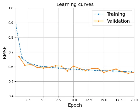

Phân tích: Cả training và validation metric đều giảm dần và tiệm cận nhau, cho thấy mô hình đang học tốt và chưa có dấu hiệu overfitting nghiêm trọng.

7. Xây dựng mô hình phi tuần tự (Nonsequential Models) sử dụng Custom Modules

nn.Sequential chỉ phù hợp cho các mạng thẳng (linear stack). Để xây dựng các kiến trúc phức tạp như ResNet hay Wide & Deep, ta cần kế thừa lớp nn.Module.

7.1. Mô hình Wide & Deep

Kiến trúc Wide & Deep (Cheng et al., 2016) kết hợp khả năng ghi nhớ (memorization) của mô hình tuyến tính (Wide) và khả năng tổng quát hóa (generalization) của mạng nơ-ron sâu (Deep).

class WideAndDeep(nn.Module):
    def __init__(self, n_features):
        super().__init__()
        # Phần "Deep"
        self.deep_stack = nn.Sequential(
            nn.Linear(n_features, 50), nn.ReLU(),
            nn.Linear(50, 40), nn.ReLU(),
            nn.Linear(40, 30), nn.ReLU(),
        )
        # Lớp đầu ra nhận input nối từ cả phần gốc (Wide) và phần Deep
        self.output_layer = nn.Linear(30 + n_features, 1)

    def forward(self, X):
        deep_output = self.deep_stack(X)
        # Nối (concat) input X và output của phần Deep lại với nhau
        wide_and_deep = torch.concat([X, deep_output], dim=1)
        return self.output_layer(wide_and_deep)

torch.manual_seed(42)
model = WideAndDeep(n_features).to(device)
learning_rate = 0.002  # Mô hình thay đổi, learning rate tối ưu có thể thay đổi

# Huấn luyện mô hình Wide & Deep
optimizer = torch.optim.SGD(model.parameters(), lr=learning_rate, momentum=0)
mse = nn.MSELoss()
rmse = torchmetrics.MeanSquaredError(squared=False).to(device)
history = train2(model, optimizer, mse, rmse, train_loader, valid_loader,
                 n_epochs)

output:
    Epoch 1/20, train loss: 1.7802, train metric: 1.3344, valid metric: 0.8690
    ...
    Epoch 20/20, train loss: 0.3834, train metric: 0.6193, valid metric: 0.5957

7.2. Xây dựng mô hình với nhiều đầu vào (Multiple Inputs)

class WideAndDeepV2(nn.Module):
    def __init__(self, n_features):
        super().__init__()
        # Giả sử ta gửi n_features - 2 đặc trưng vào nhánh Deep
        self.deep_stack = nn.Sequential(
            nn.Linear(n_features - 2, 50), nn.ReLU(),
            nn.Linear(50, 40), nn.ReLU(),
            nn.Linear(40, 30), nn.ReLU(),
        )
        # Output layer nhận 5 đặc trưng từ Wide + 30 đặc trưng từ Deep
        self.output_layer = nn.Linear(30 + 5, 1)

    def forward(self, X):
        # Cắt lát input tensor
        X_wide = X[:, :5]
        X_deep = X[:, 2:]

        deep_output = self.deep_stack(X_deep)
        wide_and_deep = torch.concat([X_wide, deep_output], dim=1)
        return self.output_layer(wide_and_deep)

torch.manual_seed(42)
model = WideAndDeepV2(n_features).to(device)

learning_rate = 0.002
optimizer = torch.optim.SGD(model.parameters(), lr=learning_rate, momentum=0)
mse = nn.MSELoss()
rmse = torchmetrics.MeanSquaredError(squared=False).to(device)
history = train2(model, optimizer, mse, rmse, train_loader, valid_loader,
                 n_epochs)

output:
    Epoch 1/20, train loss: 1.8482, train metric: 1.3598, valid metric: 0.9100
    ...
    Epoch 20/20, train loss: 0.4082, train metric: 0.6389, valid metric: 0.6493

Phiên bản nhận 2 tensor đầu vào riêng biệt:

class WideAndDeepV3(nn.Module):
    def __init__(self, n_features):
        super().__init__()
        self.deep_stack = nn.Sequential(
            nn.Linear(n_features - 2, 50), nn.ReLU(),
            nn.Linear(50, 40), nn.ReLU(),
            nn.Linear(40, 30), nn.ReLU(),
        )
        self.output_layer = nn.Linear(30 + 5, 1)

    # Hàm forward nhận 2 tham số đầu vào riêng biệt
    def forward(self, X_wide, X_deep):
        deep_output = self.deep_stack(X_deep)
        wide_and_deep = torch.concat([X_wide, deep_output], dim=1)
        return self.output_layer(wide_and_deep)

torch.manual_seed(42)
# Tạo TensorDataset với 3 thành phần: X_wide, X_deep, y
train_data_wd = TensorDataset(X_train[:, :5], X_train[:, 2:], y_train)
train_loader_wd = DataLoader(train_data_wd, batch_size=32, shuffle=True)

valid_data_wd = TensorDataset(X_valid[:, :5], X_valid[:, 2:], y_valid)
valid_loader_wd = DataLoader(valid_data_wd, batch_size=32)

test_data_wd = TensorDataset(X_test[:, :5], X_test[:, 2:], y_test)
test_loader_wd = DataLoader(test_data_wd, batch_size=32)

def evaluate_multi_in(model, data_loader, metric):
    model.eval()
    metric.reset()
    with torch.no_grad():
        for X_batch_wide, X_batch_deep, y_batch in data_loader:
            X_batch_wide = X_batch_wide.to(device)
            X_batch_deep = X_batch_deep.to(device)
            y_batch = y_batch.to(device)
            # Gọi model với 2 input
            y_pred = model(X_batch_wide, X_batch_deep)
            metric.update(y_pred, y_batch)
    return metric.compute()

def train_multi_in(model, optimizer, criterion, metric, train_loader,
                   valid_loader, n_epochs):
    history = {"train_losses": [], "train_metrics": [], "valid_metrics": []}
    for epoch in range(n_epochs):
        total_loss = 0.
        metric.reset()
        # *X_batch_inputs dùng để unpack (giải nén) nhiều input
        for *X_batch_inputs, y_batch in train_loader:
            model.train()
            X_batch_inputs = [X.to(device) for X in X_batch_inputs]
            y_batch = y_batch.to(device)
            # Gọi model với danh sách input đã unpack
            y_pred = model(*X_batch_inputs)
            loss = criterion(y_pred, y_batch)
            total_loss += loss.item()
            loss.backward()
            optimizer.step()
            optimizer.zero_grad()
            metric.update(y_pred, y_batch)

        mean_loss = total_loss / len(train_loader)
        history["train_losses"].append(mean_loss)
        history["train_metrics"].append(metric.compute().item())
        history["valid_metrics"].append(
            evaluate_multi_in(model, valid_loader, metric).item())

        print(f"Epoch {epoch + 1}/{n_epochs}, "
              f"train loss: {history['train_losses'][-1]:.4f}, "
              f"train metric: {history['train_metrics'][-1]:.4f}, "
              f"valid metric: {history['valid_metrics'][-1]:.4f}")
    return history

torch.manual_seed(42)
learning_rate = 0.01
model = WideAndDeepV3(n_features).to(device)
optimizer = torch.optim.SGD(model.parameters(), lr=learning_rate, momentum=0)
mse = nn.MSELoss()
rmse = torchmetrics.MeanSquaredError(squared=False).to(device)
history = train_multi_in(model, optimizer, mse, rmse, train_loader_wd,
                         valid_loader_wd, n_epochs)

output:
    Epoch 1/20, train loss: 0.8366, train metric: 0.9148, valid metric: 0.6892
    ...
    Epoch 20/20, train loss: 0.3414, train metric: 0.5843, valid metric: 0.5690

Sử dụng Dictionary để truyền dữ liệu rõ ràng hơn, tránh nhầm lẫn vị trí input:

class WideAndDeepDataset(torch.utils.data.Dataset):
    def __init__(self, X_wide, X_deep, y):
        self.X_wide = X_wide
        self.X_deep = X_deep
        self.y = y

    # Trả về tổng số mẫu
    def __len__(self):
        return len(self.y)

    # Lấy một mẫu tại chỉ mục idx
    def __getitem__(self, idx):
        input_dict = {"X_wide": self.X_wide[idx], "X_deep": self.X_deep[idx]}
        return input_dict, self.y[idx]

torch.manual_seed(42)
train_data_named = WideAndDeepDataset(
    X_wide=X_train[:, :5], X_deep=X_train[:, 2:], y=y_train)
train_loader_named = DataLoader(train_data_named, batch_size=32, shuffle=True)

valid_data_named = WideAndDeepDataset(
    X_wide=X_valid[:, :5], X_deep=X_valid[:, 2:], y=y_valid)
valid_loader_named = DataLoader(valid_data_named, batch_size=32)

test_data_named = WideAndDeepDataset(
    X_wide=X_test[:, :5], X_deep=X_test[:, 2:], y=y_test)
test_loader_named = DataLoader(test_data_named, batch_size=32)

def evaluate_named(model, data_loader, metric):
    model.eval()
    metric.reset()
    with torch.no_grad():
        for inputs, y_batch in data_loader:
            # inputs là một dict, ta chuyển từng value sang device
            inputs = {name: X.to(device) for name, X in inputs.items()}
            y_batch = y_batch.to(device)
            # Gọi model với keyword arguments
            y_pred = model(X_wide=inputs["X_wide"], X_deep=inputs["X_deep"])
            metric.update(y_pred, y_batch)
    return metric.compute()

def train_named(model, optimizer, criterion, metric, train_loader,
                    valid_loader, n_epochs):
    history = {"train_losses": [], "train_metrics": [], "valid_metrics": []}
    for epoch in range(n_epochs):
        total_loss = 0.
        metric.reset()
        for inputs, y_batch in train_loader:
            model.train()
            inputs = {name: X.to(device) for name, X in inputs.items()}
            y_batch = y_batch.to(device)
            # **inputs sẽ unpack dictionary thành các keyword arguments
            y_pred = model(**inputs)
            loss = criterion(y_pred, y_batch)
            total_loss += loss.item()
            loss.backward()
            optimizer.step()
            optimizer.zero_grad()
            metric.update(y_pred, y_batch)

        mean_loss = total_loss / len(train_loader)
        history["train_losses"].append(mean_loss)
        history["train_metrics"].append(metric.compute().item())
        history["valid_metrics"].append(
            evaluate_named(model, valid_loader, metric).item())

        print(f"Epoch {epoch + 1}/{n_epochs}, "
              f"train loss: {history['train_losses'][-1]:.4f}, "
              f"train metric: {history['train_metrics'][-1]:.4f}, "
              f"valid metric: {history['valid_metrics'][-1]:.4f}")
    return history

torch.manual_seed(42)
learning_rate = 0.01
model = WideAndDeepV3(n_features).to(device)
optimizer = torch.optim.SGD(model.parameters(), lr=learning_rate, momentum=0)
mse = nn.MSELoss()
rmse = torchmetrics.MeanSquaredError(squared=False).to(device)
history = train_named(model, optimizer, mse, rmse, train_loader_named,
                      valid_loader_named, n_epochs)

output:
    Epoch 1/20, train loss: 0.8366, train metric: 0.9148, valid metric: 0.6892
    ...
    Epoch 20/20, train loss: 0.3414, train metric: 0.5843, valid metric: 0.5690

7.3. Xây dựng mô hình với nhiều đầu ra (Multiple Outputs)

Kỹ thuật Auxiliary Output (Đầu ra phụ) thường được dùng để chống lại sự biến mất gradient ở các lớp sâu, hoặc để buộc các tầng ẩn học được các đặc trưng có ý nghĩa.

class WideAndDeepV4(nn.Module):
    def __init__(self, n_features):
        super().__init__()
        self.deep_stack = nn.Sequential(
            nn.Linear(n_features - 2, 50), nn.ReLU(),
            nn.Linear(50, 40), nn.ReLU(),
            nn.Linear(40, 30), nn.ReLU(),
        )
        self.output_layer = nn.Linear(30 + 5, 1)
        # Đầu ra phụ: chỉ nhận input từ nhánh Deep
        self.aux_output_layer = nn.Linear(30, 1)

    def forward(self, X_wide, X_deep):
        deep_output = self.deep_stack(X_deep)
        wide_and_deep = torch.concat([X_wide, deep_output], dim=1)
        main_output = self.output_layer(wide_and_deep)
        aux_output = self.aux_output_layer(deep_output)
        # Trả về cả 2 đầu ra
        return main_output, aux_output

Hàm Loss tổng hợp là tổng có trọng số: loss = 0.8 * main_loss + 0.2 * aux_loss.

import torchmetrics

def evaluate_multi_out(model, data_loader, metric):
    model.eval()
    metric.reset()
    with torch.no_grad():
        for inputs, y_batch in data_loader:
            inputs = {name: X.to(device) for name, X in inputs.items()}
            y_batch = y_batch.to(device)
            # Chỉ quan tâm đầu ra chính (y_pred) khi đánh giá
            y_pred, _ = model(**inputs)
            metric.update(y_pred, y_batch)
    return metric.compute()

def train_multi_out(model, optimizer, criterion, metric, train_loader,
                    valid_loader, n_epochs):
    history = {"train_losses": [], "train_metrics": [], "valid_metrics": []}
    for epoch in range(n_epochs):
        total_loss = 0.
        metric.reset()
        for inputs, y_batch in train_loader:
            model.train()
            inputs = {name: X.to(device) for name, X in inputs.items()}
            y_batch = y_batch.to(device)

            # Nhận 2 output
            y_pred, y_pred_aux = model(**inputs)

            # Tính loss cho từng output
            main_loss = criterion(y_pred, y_batch)
            aux_loss = criterion(y_pred_aux, y_batch)

            # Tổng hợp loss có trọng số
            loss = 0.8 * main_loss + 0.2 * aux_loss

            total_loss += loss.item()
            loss.backward()
            optimizer.step()
            optimizer.zero_grad()
            metric.update(y_pred, y_batch)

        mean_loss = total_loss / len(train_loader)
        history["train_losses"].append(mean_loss)
        history["train_metrics"].append(metric.compute().item())
        history["valid_metrics"].append(
            evaluate_multi_out(model, valid_loader, metric).item())

        print(f"Epoch {epoch + 1}/{n_epochs}, "
              f"train loss: {history['train_losses'][-1]:.4f}, "
              f"train metric: {history['train_metrics'][-1]:.4f}, "
              f"valid metric: {history['valid_metrics'][-1]:.4f}")
    return history

torch.manual_seed(42)
learning_rate = 0.01
model = WideAndDeepV4(n_features).to(device)
optimizer = torch.optim.SGD(model.parameters(), lr=learning_rate, momentum=0)
mse = nn.MSELoss()
rmse = torchmetrics.MeanSquaredError(squared=False).to(device)
history = train_multi_out(model, optimizer, mse, rmse, train_loader_named,
                          valid_loader_named, n_epochs)

output:
    Epoch 1/20, train loss: 1.0693, train metric: 0.9506, valid metric: 0.7085
    ...
    Epoch 20/20, train loss: 0.3566, train metric: 0.5837, valid metric: 0.5654

8. Xây dựng bộ phân loại ảnh với PyTorch (Image Classifier)

Chúng ta chuyển sang bài toán Phân loại (Classification). Sự khác biệt chính về mặt toán học nằm ở hàm loss và lớp đầu ra.

8.1. Sử dụng TorchVision để tải dữ liệu

import torchvision
import torchvision.transforms.v2 as T

# Định nghĩa pipeline biến đổi: Chuyển sang Image -> Chuyển sang Tensor float32 và scale về [0, 1]
toTensor = T.Compose([T.ToImage(), T.ToDtype(torch.float32, scale=True)])

# Tải dữ liệu huấn luyện
train_and_valid_data = torchvision.datasets.FashionMNIST(
    root="datasets", train=True, download=True, transform=toTensor)
# Tải dữ liệu kiểm tra
test_data = torchvision.datasets.FashionMNIST(
    root="datasets", train=False, download=True, transform=toTensor)

# Chia tập train thành train và validation
torch.manual_seed(42)
train_data, valid_data = torch.utils.data.random_split(
    train_and_valid_data, [55_000, 5_000])

torch.manual_seed(42)
train_loader = DataLoader(train_data, batch_size=32, shuffle=True)
valid_loader = DataLoader(valid_data, batch_size=32)
test_loader = DataLoader(test_data, batch_size=32)

X_sample, y_sample = train_data[0]

X_sample.shape # Kết quả mong đợi: torch.Size([1, 28, 28])

output:
    torch.Size([1, 28, 28])

X_sample.dtype

output:
    torch.float32

# Xem tên lớp của mẫu đầu tiên
train_and_valid_data.classes[y_sample]

output:
    'Ankle boot'

8.2. Xây dựng Bộ phân loại (Classifier)

Mạng phân loại đa lớp sử dụng hàm Softmax ở đầu ra để biến đổi logits thành phân phối xác suất: $\hat{p}_k = \frac{\exp(z_k)}{\sum_{j=1}^K \exp(z_j)}$ Và hàm mất mát Cross-Entropy: $L = -\sum_{k=1}^K y_k \log(\hat{p}_k)$ Trong PyTorch, nn.CrossEntropyLoss kết hợp cả LogSoftmax và NLLLoss để đảm bảo tính ổn định số học (tránh lỗi tràn số khi tính log). Do đó, lớp cuối của mạng không cần hàm kích hoạt.

class ImageClassifier(nn.Module):
    def __init__(self, n_inputs, n_hidden1, n_hidden2, n_classes):
        super().__init__()
        self.mlp = nn.Sequential(
            nn.Flatten(), # Duỗi phẳng ảnh 28x28 thành vector 784
            nn.Linear(n_inputs, n_hidden1),
            nn.ReLU(),
            nn.Linear(n_hidden1, n_hidden2),
            nn.ReLU(),
            nn.Linear(n_hidden2, n_classes)
        )

    def forward(self, X):
        return self.mlp(X)

torch.manual_seed(42)
model = ImageClassifier(n_inputs=1 * 28 * 28, n_hidden1=300, n_hidden2=100,
                        n_classes=10).to(device)
xentropy = nn.CrossEntropyLoss()

optimizer = torch.optim.SGD(model.parameters(), lr=0.1)
# Sử dụng Accuracy metric cho bài toán multiclass
accuracy = torchmetrics.Accuracy(task="multiclass", num_classes=10).to(device)

# Huấn luyện mô hình
_ = train2(model, optimizer, xentropy, accuracy, train_loader, valid_loader,
           n_epochs)

output:
    Epoch 1/20, train loss: 0.6058, train metric: 0.7816, valid metric: 0.8416
    ...
    Epoch 20/20, train loss: 0.1888, train metric: 0.9282, valid metric: 0.8716

Sau khi huấn luyện, dùng argmax để chọn lớp có xác suất cao nhất.

model.eval()
X_new, y_new = next(iter(valid_loader))
X_new = X_new[:3].to(device)
with torch.no_grad():
    y_pred_logits = model(X_new)

y_pred = y_pred_logits.argmax(dim=1)  # Chỉ số của logit lớn nhất
y_pred

output:
    tensor([7, 4, 2], device='cuda:0')

# Chuyển chỉ số thành tên lớp
[train_and_valid_data.classes[index] for index in y_pred]

output:
    ['Sneaker', 'Coat', 'Pullover']

y_new[:3]

output:
    tensor([7, 4, 2])

Dùng hàm softmax để xem xác suất cụ thể:

import torch.nn.functional as F

y_proba = F.softmax(y_pred_logits, dim=1)
if device == "mps":
    y_proba = y_proba.cpu() # MPS chưa hỗ trợ tốt hàm round
y_proba.round(decimals=3)

output:
    tensor([[0.0000, 0.0000, 0.0000, 0.0000, 0.0000, 0.0010, 0.0000, 0.9110, 0.0000,
             0.0880],
            [0.0000, 0.0000, 0.0040, 0.0000, 0.9960, 0.0000, 0.0000, 0.0000, 0.0000,
             0.0000],
            [0.0000, 0.0000, 0.6250, 0.0000, 0.3350, 0.0000, 0.0390, 0.0000, 0.0000,
             0.0000]], device='cuda:0')

# Lấy top 4 lớp có xác suất cao nhất
y_top4_values, y_top4_indices = torch.topk(y_pred_logits, k=4, dim=1)
y_top4_probas = F.softmax(y_top4_values, dim=1)
if device == "mps":
    y_top4_probas = y_top4_probas.cpu()
y_top4_probas.round(decimals=3)

output:
    tensor([[0.9110, 0.0880, 0.0010, 0.0000],
            [0.9960, 0.0040, 0.0000, 0.0000],
            [0.6250, 0.3350, 0.0390, 0.0000]], device='cuda:0')

y_top4_indices

output:
    tensor([[7, 9, 5, 8],
            [4, 2, 6, 0],
            [2, 4, 6, 0]], device='cuda:0')

# Đếm tổng số tham số trong mô hình
sum([param.numel() for param in model.parameters()])

output:
    266610

9. Tối ưu hóa Siêu tham số với Optuna (Hyperparameter Tuning using Optuna)

Optuna sử dụng thuật toán TPE (Tree-structured Parzen Estimator). Thay vì tìm kiếm ngẫu nhiên (Random Search) hoặc tìm kiếm lưới (Grid Search), TPE mô hình hóa xác suất $p(x|y)$ để chọn các bộ tham số có khả năng cải thiện kết quả cao nhất dựa trên lịch sử các lần chạy trước.

import optuna

def objective(trial):
    # Định nghĩa không gian tìm kiếm
    learning_rate = trial.suggest_float("learning_rate", 1e-5, 1e-1, log=True)
    n_hidden = trial.suggest_int("n_hidden", 20, 300)

    # Tạo mô hình với tham số từ trial
    model = ImageClassifier(n_inputs=1 * 28 * 28, n_hidden1=n_hidden,
                            n_hidden2=n_hidden, n_classes=10).to(device)
    optimizer = torch.optim.SGD(model.parameters(), lr=learning_rate)
    xentropy = nn.CrossEntropyLoss()
    accuracy = torchmetrics.Accuracy(task="multiclass", num_classes=10)
    accuracy = accuracy.to(device)

    # Huấn luyện nhanh (ở đây dùng 10 epochs)
    history = train2(model, optimizer, xentropy, accuracy, train_loader,
                     valid_loader, n_epochs=10)

    # Mục tiêu tối ưu hóa là validation accuracy cao nhất
    validation_accuracy = max(history["valid_metrics"])
    return validation_accuracy

torch.manual_seed(42)
# Sử dụng bộ lấy mẫu TPE (Tree-structured Parzen Estimator)
sampler = optuna.samplers.TPESampler(seed=42)
study = optuna.create_study(direction="maximize", sampler=sampler)
study.optimize(objective, n_trials=5) # Chạy 5 thử nghiệm

output:
    [I 2025-12-31 02:59:29,583] A new study created in memory with name: no-name-b54e2afc-1c7d-4d1f-a424-a0a47c9206e5
    ...
    [I 2025-12-31 03:12:04,261] Trial 4 finished with value: 0.8220000267028809 and parameters: {'learning_rate': 0.002537815508265664, 'n_hidden': 218}. Best is trial 1 with value: 0.8547999858856201.

# Các tham số tốt nhất tìm được
study.best_params

output:
    {'learning_rate': 0.008471801418819975, 'n_hidden': 188}

# Giá trị accuracy tốt nhất
study.best_value

output:
    0.8547999858856201

Kỹ thuật Pruning (Cắt tỉa) cho phép dừng sớm các thử nghiệm kém triển vọng, tiết kiệm tài nguyên tính toán.

def objective(trial, train_loader, valid_loader):
    learning_rate = trial.suggest_float("learning_rate", 1e-5, 1e-1, log=True)
    n_hidden = trial.suggest_int("n_hidden", 20, 300)
    model = ImageClassifier(n_inputs=1 * 28 * 28, n_hidden1=n_hidden,
                            n_hidden2=n_hidden, n_classes=10).to(device)
    optimizer = torch.optim.SGD(model.parameters(), lr=learning_rate)
    xentropy = nn.CrossEntropyLoss()
    accuracy = torchmetrics.Accuracy(task="multiclass", num_classes=10)
    accuracy = accuracy.to(device)

    best_validation_accuracy = 0.0
    for epoch in range(n_epochs):
        history = train2(model, optimizer, xentropy, accuracy, train_loader,
                         valid_loader, n_epochs=1)
        validation_accuracy = max(history["valid_metrics"])
        if validation_accuracy > best_validation_accuracy:
            best_validation_accuracy = validation_accuracy

        # Báo cáo kết quả hiện tại cho Optuna
        trial.report(validation_accuracy, epoch)
        # Nếu kết quả quá tệ, dừng sớm (pruning)
        if trial.should_prune():
            raise optuna.TrialPruned()
    return best_validation_accuracy

# Sử dụng partial để truyền sẵn tham số train_loader và valid_loader
from functools import partial

objective_with_data = partial(objective, train_loader=train_loader,
                              valid_loader=valid_loader)

torch.manual_seed(42)
sampler = optuna.samplers.TPESampler(seed=42)
# Sử dụng MedianPruner: cắt bỏ các trial kém hơn mức trung vị của các trial trước đó
pruner = optuna.pruners.MedianPruner()
study = optuna.create_study(direction="maximize", sampler=sampler,
                            pruner=pruner)
study.optimize(objective_with_data, n_trials=20)

output:
    [I 2025-12-31 03:12:04,298] A new study created in memory with name: no-name-cd938a39-9a4a-47ab-8401-aa962c976b13
    ...
    [I 2025-12-31 04:14:54,231] Trial 19 pruned. 

study.best_value

output:
    0.8867999911308289

study.best_params

output:
    {'learning_rate': 0.08525846269447772, 'n_hidden': 116}

10. Lưu và Tải mô hình PyTorch (Saving and Loading)

# Cách 1: Lưu toàn bộ mô hình (Pickle) - Không khuyến nghị cho production
torch.save(model, "my_fashion_mnist.pt")

# Tải lại toàn bộ mô hình
loaded_model = torch.load("my_fashion_mnist.pt", weights_only=False)

loaded_model.eval()
y_pred_logits = loaded_model(X_new)

State Dict là cách lưu trữ chuẩn, chỉ lưu các tham số (weights & biases) dưới dạng Ordered Dictionary.

# Cách 2: Chỉ lưu state_dict (khuyến nghị)
torch.save(model.state_dict(), "my_fashion_mnist_weights.pt")

# state_dict thực chất là một OrderDict ánh xạ tên tham số -> tensor
type(model.state_dict())

output:
    collections.OrderedDict

# Để tải lại, ta cần khởi tạo mô hình trước, sau đó load trọng số vào
new_model = ImageClassifier(n_inputs=1 * 28 * 28, n_hidden1=300, n_hidden2=100,
                            n_classes=10)
loaded_weights = torch.load("my_fashion_mnist_weights.pt", weights_only=True)
new_model.load_state_dict(loaded_weights)
new_model.eval()

output:
    ImageClassifier(
      (mlp): Sequential(...)
    )

model_data = {
    "model_state_dict": model.state_dict(),
    "model_hyperparameters": {
        "n_inputs": 1 * 28 * 28,
        "n_hidden1": 300,
        "n_hidden2": 100,
        "n_classes": 10,
    }
}
torch.save(model_data, "my_fashion_mnist_model.pt")

loaded_data = torch.load("my_fashion_mnist_model.pt", weights_only=True)
# Khởi tạo mô hình dùng siêu tham số đã lưu
new_model = ImageClassifier(**loaded_data["model_hyperparameters"])
# Load trọng số
new_model.load_state_dict(loaded_data["model_state_dict"])
new_model.eval()

output:
    ImageClassifier(
      (mlp): Sequential(...)
    )

11. Biên dịch và Tối ưu hóa Mô hình (Compiling and Optimizing)

TorchScript (JIT): Chuyển đổi mô hình Python động thành đồ thị tĩnh trung gian (Intermediate Representation - IR), cho phép chạy trong môi trường C++ hiệu năng cao.

# Cách 1: Tracing (Theo vết)
# Chạy mô hình với một input giả định và ghi lại các phép toán đã thực hiện
torchscript_model = torch.jit.trace(model, X_new)

# Cách 2: Scripting
# Phân tích mã nguồn Python để chuyển đổi. Hỗ trợ control flow (if/else, loop)
torchscript_model = torch.jit.script(model)

# Tối ưu hóa mô hình cho suy luận (inference) - Gộp các lớp (Layer Fusion)
optimized_model = torch.jit.optimize_for_inference(torchscript_model)

# Lưu mô hình TorchScript
optimized_model.save("my_fashion_mnist_torchscript.pt")

# Tải lại mô hình TorchScript
loaded_torchscript_model = torch.jit.load("my_fashion_mnist_torchscript.pt")

y_pred_logits = loaded_torchscript_model(X_new)
y_pred_logits

output:
    tensor([[ -3.3324,  -0.7572,  -4.1671,  -1.9444,  -1.6955,   2.0123,  -3.2624,
               8.6379,  -0.5685,   6.2972],
            ...], device='cuda:0')

torch.compile: Tính năng mới trong PyTorch 2.0, tối ưu hóa đồ thị động thành các kernel triton tối ưu.

compiled_model = torch.compile(model)

# Lưu ý: torch.compile hiện tại chủ yếu hỗ trợ tốt trên CUDA (Linux) và chưa hỗ trợ tốt Windows/MPS
if device == "cuda":
    y_pred_logits = compiled_model(X_new)

12. Ôn tập & Bài tập Thực hành

Bài tập 1: Tính đạo hàm riêng

Yêu cầu: Sử dụng autograd để tìm vector gradient của hàm $f(x, y) = \sin(x^2 y)$ tại điểm $(x, y) = (1.2, 3.4)$.

Về mặt giải tích: $\frac{\partial f}{\partial x} = \cos(x^2 y) \cdot 2xy$ $\frac{\partial f}{\partial y} = \cos(x^2 y) \cdot x^2$

def f(x, y):
    return torch.sin(x ** 2 * y)

x = torch.tensor(1.2, requires_grad=True)
y = torch.tensor(3.4, requires_grad=True)
result = f(x, y)
result.backward()

x.grad.item(), y.grad.item()

output:
    (1.489864706993103, 0.26291730999946594)

Kiểm tra lại bằng sai phân hữu hạn (Numerical Differentiation):

eps = 0.00005
df_dx = (f(x + eps, y) - f(x, y)) / eps
df_dy = (f(x, y + eps) - f(x, y)) / eps

df_dx.item(), df_dy.item()

output:
    (1.4901161193847656, 0.26226043701171875)

Tính toán chính xác theo công thức:

df_dx = 2 * x * y * torch.cos(x**2 * y)
df_dy = x ** 2 * torch.cos(x**2 * y)

df_dx.item(), df_dy.item()

output:
    (1.4898648262023926, 0.26291730999946594)

Bài tập 2: Custom Module Dense

Yêu cầu: Tạo một module Dense tùy chỉnh mô phỏng chức năng của một module nn.Linear theo sau bởi nn.ReLU.

class Dense(nn.Module):
    def __init__(self, in_features, out_features):
        super().__init__()
        # Sử dụng lại các module có sẵn
        self.linear = nn.Linear(in_features, out_features)
        self.relu = nn.ReLU()

    def forward(self, X):
        return self.relu(self.linear(X))

torch.manual_seed(42)
dense = Dense(3, 5)
X = torch.randn(2, 3)
y_pred = dense(X)
y_pred.shape

output:
    torch.Size([2, 5])

# Kiểm tra tính chính xác
y_pred_check = dense.relu(X @ dense.linear.weight.T + dense.linear.bias)
torch.allclose(y_pred, y_pred_check)

output:
    True

Phiên bản nâng cao sử dụng nn.Parameter để quản lý trọng số thủ công:

class Dense2(nn.Module):
    def __init__(self, in_features, out_features):
        super().__init__()
        # nn.Parameter báo cho PyTorch biết đây là tham số cần huấn luyện
        self.weight = nn.Parameter(torch.randn(out_features, in_features))
        self.bias = nn.Parameter(torch.zeros(out_features))

    def forward(self, X):
        z = X @ self.weight.T + self.bias
        return F.relu(z)

import torch.nn.functional as F

torch.manual_seed(42)
dense2 = Dense2(3, 5)
X = torch.randn(2, 3)
y_pred2 = dense2(X)
y_pred2.shape

output:
    torch.Size([2, 5])

y_pred2_check = F.relu(X @ dense2.weight.T + dense2.bias)
torch.allclose(y_pred2, y_pred2_check)

output:
    True

Khởi tạo Kaiming Uniform (He Initialization) để tối ưu cho ReLU:

class Dense3(nn.Module):
    def __init__(self, in_features, out_features):
        super().__init__()
        self.weight = nn.Parameter(torch.empty(out_features, in_features))
        # Khởi tạo Kaiming Uniform
        nn.init.kaiming_uniform_(self.weight, nonlinearity="relu")
        self.bias = nn.Parameter(torch.zeros(out_features))

    def forward(self, X):
        z = X @ self.weight.T + self.bias
        return F.relu(z)

torch.manual_seed(42)
dense3 = Dense3(3, 5)
X = torch.randn(2, 3)
y_pred3 = dense3(X)
y_pred3.shape

output:
    torch.Size([2, 5])

y_pred3_check = F.relu(X @ dense3.weight.T + dense3.bias)
torch.allclose(y_pred3, y_pred3_check)

output:
    True

Bài tập 3: Phân loại bộ dữ liệu CoverType

Yêu cầu: Xây dựng và huấn luyện một MLP phân loại trên bộ dữ liệu CoverType. Đây là bộ dữ liệu lớn (581k mẫu) với 54 đặc trưng và 7 lớp mục tiêu.

"""
# Cách nhanh nhất để tải dataset này là:
from sklearn.datasets import fetch_covtype
from torch.utils.data import TensorDataset
covtype = fetch_covtype()
# Tuy nhiên, ở thời điểm viết bài này, link tải dataset thô đã bị thay đổi
# và Sklearn chưa cập nhật điều này.
# Vì vậy, tạm thời chúng ta sẽ dùng cách tải và xử lý thủ công như sau.
"""

import os
import gzip
import numpy as np
import urllib.request
from sklearn.utils import Bunch

def fetch_covtype_fixed(data_home=None, download_if_missing=True):
    """
    A workaround for sklearn.datasets.fetch_covtype using a working URL.
    Returns the same Bunch object structure.
    """

    # 1. Setup Paths and URL
    # We use the user-verified working link
    URL = "https://figshare.com/ndownloader/files/5976039"
    ARCHIVE_NAME = "covtype.data.gz"

    # Use a local directory to cache the file so we don't download it every time
    if data_home is None:
        data_home = os.path.join(os.getcwd(), "scikit_learn_data_custom")

    if not os.path.exists(data_home):
        os.makedirs(data_home)

    archive_path = os.path.join(data_home, ARCHIVE_NAME)

    # 2. Download the data if it doesn't exist
    if not os.path.exists(archive_path):
        if download_if_missing:
            print(f"Downloading data from {URL} to {archive_path}...")
            try:
                urllib.request.urlretrieve(URL, archive_path)
                print("Download complete.")
            except Exception as e:
                raise RuntimeError(f"Failed to download data: {e}")
        else:
            raise IOError("Data not found and download_if_missing is False")
    else:
        print(f"Found cached data at {archive_path}")

    # 3. Load and Process Data
    print("Loading data into memory (this may take a moment)...")

    # We use numpy directly to match sklearn's original behavior
    # This reads the compressed CSV directly
    with gzip.open(archive_path, 'rb') as f:
        Xy = np.genfromtxt(f, delimiter=',')

    # The last column is the target (Cover_Type)
    X = Xy[:, :-1]
    y = Xy[:, -1].astype(np.int32)

    # 4. Construct Metadata (Feature Names)
    # Copied exactly from the sklearn source code provided
    FEATURE_NAMES = [
        "Elevation",
        "Aspect",
        "Slope",
        "Horizontal_Distance_To_Hydrology",
        "Vertical_Distance_To_Hydrology",
        "Horizontal_Distance_To_Roadways",
        "Hillshade_9am",
        "Hillshade_Noon",
        "Hillshade_3pm",
        "Horizontal_Distance_To_Fire_Points",
    ]
    FEATURE_NAMES += [f"Wilderness_Area_{i}" for i in range(4)]
    FEATURE_NAMES += [f"Soil_Type_{i}" for i in range(40)]
    TARGET_NAMES = ["Cover_Type"]

    # 5. Return the Bunch object (Identical structure to sklearn)
    return Bunch(
        data=X,
        target=y,
        feature_names=FEATURE_NAMES,
        target_names=TARGET_NAMES,
        DESCR="Forest covertype dataset (Workaround Version)",
        frame=None # Set to None for compatibility, or construct a DF if needed
    )

# Get the variable exactly as you wanted
covtype = fetch_covtype_fixed()

output:
    Found cached data at /content/scikit_learn_data_custom/covtype.data.gz
    Loading data into memory (this may take a moment)...

from torch.utils.data import TensorDataset, DataLoader

# Chuyển sang tensor float32
X_covtype = torch.tensor(covtype.data, dtype=torch.float32)

# Chuẩn hóa dữ liệu (Z-score normalization)
means = X_covtype.mean(dim=0, keepdim=True)
stds = X_covtype.std(dim=0, keepdim=True)
X_standardized_covtype = (X_covtype - means) / stds

# Target trong dataset gốc từ 1-7, cần chuyển về 0-6 cho CrossEntropyLoss
y_covtype = torch.tensor(covtype.target - 1, dtype=torch.long)

covtype_dataset = TensorDataset(X_standardized_covtype, y_covtype)

sample0, target0 = covtype_dataset[0]
sample0.shape, target0.shape

output:
    (torch.Size([54]), torch.Size([]))

from torch.utils.data import random_split

torch.manual_seed(42)

# Tỷ lệ split: 80% train, 10% valid, 10% test
train_size = len(covtype_dataset) * 80 // 100
valid_size = len(covtype_dataset) * 10 // 100
test_size = len(covtype_dataset) - train_size - valid_size

train_dataset, valid_dataset, test_dataset = random_split(
    covtype_dataset,
    [train_size, valid_size, test_size])

from torch.utils.data import DataLoader

batch_size = 256 # Batch size lớn hơn một chút vì dữ liệu dạng bảng

train_loader = DataLoader(train_dataset, batch_size=batch_size, shuffle=True)
valid_loader = DataLoader(valid_dataset, batch_size=batch_size)
test_loader = DataLoader(test_dataset, batch_size=batch_size)

Xây dựng mô hình với số lượng lớp và neuron linh hoạt:

import torch.nn as nn

# Kiểm tra thiết bị khả dụng: CUDA (Nvidia GPU), MPS (Apple Silicon), hay CPU
if torch.cuda.is_available():
    device = "cuda"
elif torch.backends.mps.is_available():
    device = "mps"
else:
    device = "cpu"

n_inputs = len(covtype.feature_names)  # == 54
n_classes = len(set(covtype.target))  # == 7

class CoverTypeModel(nn.Module):
    def __init__(self, n_neurons, n_inputs=n_inputs, n_classes=n_classes):
        super().__init__()
        # Tạo danh sách các layer dựa trên cấu hình n_neurons truyền vào
        layers = [
            Dense3(n_in, n_out)
            for n_in, n_out in zip([n_inputs] + n_neurons, n_neurons)
        ] + [nn.Linear(n_neurons[-1], n_classes)] # Lớp cuối không có activation
        self.mlp = nn.Sequential(*layers)

    def forward(self, X):
        return self.mlp(X)

torch.manual_seed(42)
covtype_model = CoverTypeModel([200, 100, 50]).to(device)

Huấn luyện với chiến lược giảm dần Learning Rate (LR Decay) thủ công để tinh chỉnh hội tụ.

%pip install -q optuna torchmetrics
import torch

torch.manual_seed(42)
covtype_model = CoverTypeModel([200, 100, 50]).to(device)

# Giảm dần learning rate qua các giai đoạn
for learning_rate in [0.16, 0.08, 0.04, 0.02, 0.01, 0.005]:
    n_epochs = 15
    optimizer = torch.optim.SGD(covtype_model.parameters(), lr=learning_rate)
    criterion = nn.CrossEntropyLoss()
    metric = torchmetrics.Accuracy(task="multiclass",
                                   num_classes=n_classes).to(device)
    history = train2(covtype_model, optimizer, criterion, metric, train_loader,
                     valid_loader, n_epochs)

output:
    Epoch 1/15, train loss: 0.5829, train metric: 0.7499, valid metric: 0.7913
    ...
    Epoch 15/15, train loss: 0.0987, train metric: 0.9629, valid metric: 0.9497

# Đánh giá trên tập Test
evaluate_tm(covtype_model, test_loader, metric)

output:
    tensor(0.9489, device='cuda:0')

Sử dụng Optuna để tự động tìm kiến trúc mạng tối ưu.

Lưu ý: Để minh họa và tiết kiệm thời gian, đoạn code dưới đây thiết lập n_trials=2, và do đó sẽ cho kết quả không như mong đợi. Để đạt độ chính xác cao hơn, hãy thử tăng n_trials lên 50 hoặc hơn. Tất nhiên, thời gian chạy sẽ tăng lên đáng kể.

def objective(trial):
    learning_rate = trial.suggest_float("learning_rate", 1e-2, 1.0, log=True)
    n_layers = trial.suggest_int("n_layers", 1, 3)
    n_hidden = trial.suggest_int("n_hidden", 30, 150)

    # Tạo mô hình với cấu hình động
    covtype_model = CoverTypeModel([n_hidden] * n_layers).to(device)
    optimizer = torch.optim.SGD(covtype_model.parameters(), lr=learning_rate)
    xentropy = nn.CrossEntropyLoss()
    accuracy = torchmetrics.Accuracy(task="multiclass",
                                     num_classes=n_classes).to(device)
    best_validation_accuracy = 0.0
    for epoch in range(n_epochs):
        history = train2(covtype_model, optimizer, xentropy, accuracy,
                         train_loader, valid_loader, n_epochs=1)
        validation_accuracy = max(history["valid_metrics"])
        if validation_accuracy > best_validation_accuracy:
            best_validation_accuracy = validation_accuracy
        trial.report(validation_accuracy, step=epoch)
        if trial.should_prune():
            raise optuna.TrialPruned()
    return best_validation_accuracy

torch.manual_seed(42)
sampler = optuna.samplers.TPESampler(seed=42)
pruner = optuna.pruners.MedianPruner()
study = optuna.create_study(direction="maximize", sampler=sampler,
                            pruner=pruner)
study.optimize(objective, n_trials=2) # Tăng n_trials nếu có thời gian

output:
    [I 2025-12-31 04:26:31,661] A new study created in memory with name: no-name-14978ccc-4b62-43a2-b481-9c600fbda005
    ...
    [I 2025-12-31 04:30:10,177] Trial 1 finished with value: 0.8006230592727661 and parameters: {'learning_rate': 0.15751320499779725, 'n_layers': 1, 'n_hidden': 48}. Best is trial 0 with value: 0.8718094229698181.

study.best_value

output:
    0.8718094229698181

study.best_params

output:
    {'learning_rate': 0.05611516415334506, 'n_layers': 3, 'n_hidden': 118}

Với độ chính xác đạt gần 95% trên tập test, mô hình MLP tùy chỉnh của chúng ta đã chứng minh hiệu quả vượt trội trong việc xử lý dữ liệu bảng (tabular data).