[DL101] Chương 10: Autoencoders, GANs, và Diffusion Models

Bài viết có tham khảo, sử dụng và sửa đổi tài nguyên từ kho lưu trữ handson-mlp, tuân thủ giấy phép Apache‑2.0. Chúng tôi chân thành cảm ơn tác giả Aurélien Géron (@aureliengeron) vì sự chia sẻ kiến thức tuyệt vời và những đóng góp quý giá cho cộng đồng.

Khác với các mô hình Discriminative (Phân biệt) mà chúng ta đã tìm hiểu trước đây (như phân loại ảnh, dự đoán giá nhà) - nơi mô hình học cách ánh xạ từ đầu vào $X$ sang nhãn $y$ ($P(y|x)$), các mô hình Generative tập trung vào việc học phân phối xác suất của dữ liệu đầu vào $P(X)$ (hoặc $P(X, y)$). Mục tiêu là để hiểu cấu trúc nội tại của dữ liệu và từ đó có thể sinh ra các mẫu dữ liệu mới giống với dữ liệu thật.

Chúng ta sẽ đi qua ba kiến trúc nền tảng:

1. Autoencoders (Mạng tự mã hóa): Học cách nén dữ liệu vào một không gian biểu diễn (latent space) và khôi phục lại nó. Chúng ta sẽ khám phá các biến thể như Sparse, Denoising và Variational Autoencoders (VAE).
2. Generative Adversarial Networks (GANs - Mạng đối nghịch tạo sinh): Một cuộc chơi giữa hai mạng (Generator và Discriminator) để tạo ra dữ liệu chân thực.
3. Diffusion Models (Mô hình khuếch tán): Kiến trúc hiện đại đang thống trị lĩnh vực tạo sinh ảnh (như DALL-E, Stable Diffusion) dựa trên nguyên lý nhiệt động lực học và quá trình khử nhiễu tuần tự.

Bạn có thể chạy trực tiếp các đoạn mã code tại: Google Colab.

Cài đặt môi trường (Setup)

Trước khi đi vào lý thuyết và thực hành, chúng ta cần thiết lập môi trường làm việc. Các mô hình tạo sinh, đặc biệt là GANs và Diffusion, đòi hỏi năng lực tính toán lớn, do đó việc sử dụng GPU là gần như bắt buộc.

Dự án này yêu cầu Python phiên bản 3.10 trở lên để đảm bảo tương thích với các thư viện PyTorch mới nhất.

import sys

# Kiểm tra phiên bản Python
assert sys.version_info >= (3, 10)

Chúng ta cần xác định môi trường chạy code là Google Colab hay Kaggle để cài đặt các thư viện phụ thuộc phù hợp.

IS_COLAB = "google.colab" in sys.modules
IS_KAGGLE = "kaggle_secrets" in sys.modules

Nếu đang sử dụng Google Colab, thư viện torchmetrics (dùng để tính toán các chỉ số đánh giá mô hình) chưa được cài đặt sẵn, vì vậy chúng ta cần cài đặt thủ công.

if IS_COLAB:
    %pip install -q torchmetrics

output:
     [?25l    [90m━━━━━━━━━━━━━━━━━━━━━━━━━━━━━━━━━━━━━━━━ [0m  [32m0.0/983.2 kB [0m  [31m? [0m eta  [36m-:--:-- [0m
 [2K    [91m━━━━━━━━━━━━━━━━━━━━━━━━━━━━━━━━━━━━━━━ [0m [91m╸ [0m  [32m983.0/983.2 kB [0m  [31m39.5 MB/s [0m eta  [36m0:00:01 [0m
 [2K    [90m━━━━━━━━━━━━━━━━━━━━━━━━━━━━━━━━━━━━━━━━ [0m  [32m983.2/983.2 kB [0m  [31m22.1 MB/s [0m eta  [36m0:00:00 [0m
     [?25h

Đảm bảo rằng PyTorch phiên bản 2.6.0 hoặc mới hơn đang được sử dụng để tận dụng các tính năng tối ưu hóa mới nhất.

from packaging.version import Version
import torch

assert Version(torch.__version__) >= Version("2.6.0")

Chương này liên quan đến việc huấn luyện các mạng nơ-ron sâu và phức tạp. Nếu không có bộ tăng tốc phần cứng (Hardware Accelerator), quá trình này sẽ rất chậm. Đoạn code dưới đây sẽ tự động phát hiện và lựa chọn thiết bị tốt nhất có sẵn (cuda cho Nvidia GPU, mps cho Apple Silicon, hoặc cpu).

if torch.cuda.is_available():
    device = "cuda"
elif torch.backends.mps.is_available():
    device = "mps"
else:
    device = "cpu"

device

output:
    'cuda'

Cảnh báo người dùng nếu không tìm thấy GPU, vì việc huấn luyện trên CPU có thể không khả thi về mặt thời gian.

if device == "cpu":
    print("Neural nets can be very slow without a hardware accelerator.")
    if IS_COLAB:
        print("Go to Runtime > Change runtime and select a GPU hardware "
              "accelerator.")
    if IS_KAGGLE:
        print("Go to Settings > Accelerator and select GPU.")

Để đảm bảo các biểu đồ trực quan hóa dữ liệu được rõ ràng và thẩm mỹ, chúng ta thiết lập kích thước font chữ mặc định cho thư viện matplotlib.

import matplotlib.pyplot as plt

plt.rc('font', size=14)
plt.rc('axes', labelsize=14, titlesize=14)
plt.rc('legend', fontsize=14)
plt.rc('xtick', labelsize=10)
plt.rc('ytick', labelsize=10)

Chúng ta sẽ tái sử dụng các hàm train() và evaluate_tm() từ các chương trước để quản lý vòng lặp huấn luyện. Tuy nhiên, có một số cải tiến nhỏ:

• Gradient Clipping: Sử dụng torch.nn.utils.clip_grad_norm_() để ngăn chặn hiện tượng bùng nổ gradient (exploding gradients), thường gặp trong RNN hoặc các mạng sâu.
• Hỗ trợ đầu ra phức tạp: Hàm hỗ trợ các mô hình trả về namedtuple (ví dụ: trả về cả output và latent vector), giúp linh hoạt hơn cho các kiến trúc như VAE hay Sparse AE.

import torchmetrics

def evaluate_tm(model, data_loader, metric):
    model.eval() # Chuyển sang chế độ đánh giá
    metric.reset()
    with torch.no_grad(): # Tắt tính toán gradient
        for X_batch, y_batch in data_loader:
            X_batch, y_batch = X_batch.to(device), y_batch.to(device)
            y_pred = model(X_batch)
            # Xử lý nếu output là một tuple (dành cho các model phức tạp)
            if isinstance(y_pred, tuple):
                y_pred = y_pred.output
            metric.update(y_pred, y_batch)
    return metric.compute()

def train(model, optimizer, loss_fn, metric, train_loader, valid_loader,
          n_epochs, patience=2, factor=0.5, epoch_callback=None):
    # Scheduler để giảm learning rate khi validation metric không cải thiện
    scheduler = torch.optim.lr_scheduler.ReduceLROnPlateau(
        optimizer, mode="max", patience=patience, factor=factor)
    history = {"train_losses": [], "train_metrics": [], "valid_metrics": []}
    for epoch in range(n_epochs):
        total_loss = 0.0
        metric.reset()
        model.train() # Chuyển sang chế độ huấn luyện
        if epoch_callback is not None:
            epoch_callback(model, epoch)
        for index, (X_batch, y_batch) in enumerate(train_loader):
            X_batch, y_batch = X_batch.to(device), y_batch.to(device)
            y_pred = model(X_batch)
            loss = loss_fn(y_pred, y_batch)
            total_loss += loss.item()
            loss.backward() # Lan truyền ngược
            # Gradient clipping để ổn định huấn luyện
            torch.nn.utils.clip_grad_norm_(model.parameters(), max_norm=1.0)
            optimizer.step() # Cập nhật trọng số
            optimizer.zero_grad()
            if isinstance(y_pred, tuple):
                y_pred = y_pred.output
            metric.update(y_pred, y_batch)
            train_metric = metric.compute().item()
            # In tiến độ
            print(f"\rBatch {index + 1}/{len(train_loader)}", end="")
            print(f", loss={total_loss/(index+1):.4f}", end="")
            print(f", {train_metric=:.3f}", end="")
        history["train_losses"].append(total_loss / len(train_loader))
        history["train_metrics"].append(train_metric)
        val_metric = evaluate_tm(model, valid_loader, metric).item()
        history["valid_metrics"].append(val_metric)
        scheduler.step(val_metric)
        print(f"\rEpoch {epoch + 1}/{n_epochs},                      "
              f"train loss: {history['train_losses'][-1]:.4f}, "
              f"train metric: {history['train_metrics'][-1]:.3}, "
              f"valid metric: {history['valid_metrics'][-1]:.3}")
    return history

1. Thực hiện PCA với Undercomplete Linear Autoencoder

Lý thuyết nền tảng

Autoencoder (AE) là một mạng nơ-ron học cách sao chép đầu vào ra đầu ra. Nó bao gồm hai phần chính:

1. Encoder (Bộ mã hóa): Ánh xạ đầu vào $x$ sang một mã (code) trung gian $z = f(x)$. Không gian chứa $z$ gọi là Latent space (Không gian tiềm ẩn).
2. Decoder (Bộ giải mã): Ánh xạ mã $z$ quay trở lại không gian dữ liệu gốc $\hat{x} = g(z)$.

Mục tiêu là tối thiểu hóa sự sai khác giữa đầu vào và đầu ra tái tạo: $L(x, g(f(x)))$.

Nếu lớp ẩn (latent layer) có số chiều nhỏ hơn đầu vào, ta gọi đó là Undercomplete Autoencoder. Mạng buộc phải học các đặc trưng quan trọng nhất của dữ liệu để nén nó lại.

Mối liên hệ với PCA (Principal Component Analysis): Nếu một Autoencoder chỉ sử dụng các hàm kích hoạt tuyến tính (Linear activation) và hàm mất mát là Mean Squared Error (MSE), thì nó thực chất đang thực hiện Phân tích thành phần chính (PCA). Nó sẽ chiếu dữ liệu lên một siêu phẳng có chiều thấp hơn sao cho phương sai được giữ lại là lớn nhất (tương tự như tìm các eigenvectors).

Dưới đây, chúng ta xây dựng một Autoencoder đơn giản nhất: Tuyến tính hoàn toàn. Encoder nén dữ liệu 3D xuống 2D, và Decoder khôi phục lại 3D.

import torch
import torch.nn as nn

torch.manual_seed(42)
# Encoder: 3 chiều -> 2 chiều
encoder = nn.Linear(3, 2)
# Decoder: 2 chiều -> 3 chiều
decoder = nn.Linear(2, 3)
# Ghép nối thành Autoencoder
autoencoder = nn.Sequential(encoder, decoder).to(device)

Chúng ta sẽ tạo ra một tập dữ liệu 3D nhân tạo (giống như trong chương về Giảm chiều dữ liệu). Dữ liệu này nằm rải rác gần một mặt phẳng 2D trong không gian 3D.

# Code tạo dữ liệu 3D hình oval (tương tự [ML101] Chương 7)

import numpy as np
from scipy.spatial.transform import Rotation

def generate_data(m, seed=42):
    X = np.zeros((m, 3))  # Khởi tạo dataset 3D
    rng = np.random.default_rng(seed)
    angles = (rng.random(m) ** 3 + 0.5) * 2 * np.pi  # Phân phối không đều
    X[:, 0], X[:, 1] = np.cos(angles), np.sin(angles) * 0.5  # Hình oval
    X += 0.28 * rng.standard_normal((m, 3))  # Thêm nhiễu
    # Xoay dữ liệu
    X = Rotation.from_rotvec([np.pi / 29, -np.pi / 20, np.pi / 4]).apply(X)
    X += [0.2, 0, 0.2]  # Dịch chuyển vị trí
    return torch.from_numpy(X.astype(np.float32))

from torch.utils.data import DataLoader, TensorDataset

# Tạo tập train
X_train = generate_data(60, seed=42)
train_set = TensorDataset(X_train, X_train) # Input và Target đều là X_train (Unsupervised)
train_loader = DataLoader(train_set, batch_size=32, shuffle=True)

# Tạo tập validation
X_valid = generate_data(500, seed=43)
valid_set = TensorDataset(X_valid, X_valid)
valid_loader = DataLoader(valid_set, batch_size=32)

Tiến hành huấn luyện mô hình. Lưu ý rằng đầu ra mong muốn (y_batch) chính là đầu vào (X_batch), vì đây là học không giám sát (unsupervised learning) với mục tiêu tái tạo.

import torchmetrics

torch.manual_seed(42)
optimizer = torch.optim.NAdam(autoencoder.parameters(), lr=0.2)
mse = nn.MSELoss()
rmse = torchmetrics.MeanSquaredError(squared=False).to(device)

# Huấn luyện 20 epochs
history = train(autoencoder, optimizer, mse, rmse, train_loader, valid_loader,
                n_epochs=20)

output:
    
    Batch 1/2, loss=0.1990, train_metric=0.446
    Batch 2/2, loss=0.1621, train_metric=0.406
    Epoch 1/20,                      train loss: 0.1621, train metric: 0.406, valid metric: 0.309
    ...
    Epoch 20/20,                      train loss: 0.0283, train metric: 0.169, valid metric: 0.202

Sau khi huấn luyện, ta có thể trích xuất các vector trong không gian tiềm ẩn (Latent vectors) bằng cách cho dữ liệu đi qua encoder. Kết quả thu được chính là hình chiếu 2D của dữ liệu 3D, tương tự như PCA.

codings = encoder(X_train.to(device))

fig = plt.figure(figsize=(4,3))
codings_np = codings.cpu().detach().numpy()
plt.plot(codings_np[:,0], codings_np[:, 1], "b.")
plt.xlabel("$z_1$", fontsize=18)
plt.ylabel("$z_2$", fontsize=18, rotation=0)
plt.grid(True)

plt.show()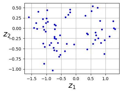

2. Stacked Autoencoders (Deep Autoencoders)

Lý thuyết

Thay vì chỉ có một lớp ẩn đơn giản, chúng ta có thể chồng nhiều lớp ẩn lên nhau để tạo thành Stacked Autoencoder (hoặc Deep Autoencoder). Việc tăng chiều sâu cho phép mô hình học các đặc trưng phức tạp hơn theo cấp bậc (hierarchical features).

Kiến trúc thường đối xứng qua lớp code ở giữa (lớp có số chiều nhỏ nhất). Ví dụ: $784 \to 128 \to 64 \to 32 \to 64 \to 128 \to 784$.

Cài đặt Stacked Autoencoder với PyTorch

Chúng ta sẽ xây dựng một Stacked AE để nén ảnh Fashion MNIST (28x28 pixel) xuống còn vector 32 chiều.

torch.manual_seed(42)  # Đảm bảo tính tái lập

# Encoder: Nén dần từ 784 -> 128 -> 32
stacked_encoder = nn.Sequential(
    nn.Flatten(),
    nn.Linear(1 * 28 * 28, 128), nn.ReLU(),
    nn.Linear(128, 32), nn.ReLU(),
)
# Decoder: Giải nén dần từ 32 -> 128 -> 784
stacked_decoder = nn.Sequential(
    nn.Linear(32, 128), nn.ReLU(),
    nn.Linear(128, 1 * 28 * 28), nn.Sigmoid(), # Sigmoid đưa giá trị về [0, 1]
    nn.Unflatten(dim=1, unflattened_size=(1, 28, 28))
)
stacked_ae = nn.Sequential(stacked_encoder, stacked_decoder).to(device)

Tải dữ liệu Fashion MNIST và chuẩn bị Data Loader.

import torchvision
import torchvision.transforms.v2 as T

toTensor = T.Compose([T.ToImage(), T.ToDtype(torch.float32, scale=True)])

# Tải dataset
train_and_valid_data = torchvision.datasets.FashionMNIST(
    root="datasets", train=True, download=True, transform=toTensor)
test_data = torchvision.datasets.FashionMNIST(
    root="datasets", train=False, download=True, transform=toTensor)

torch.manual_seed(42)
# Chia tập train/valid
train_data, valid_data = torch.utils.data.random_split(
    train_and_valid_data, [55_000, 5_000])

output:
    100%|██████████| 26.4M/26.4M [00:02<00:00, 9.52MB/s]
    100%|██████████| 29.5k/29.5k [00:00<00:00, 204kB/s]
    100%|██████████| 4.42M/4.42M [00:01<00:00, 3.79MB/s]
    100%|██████████| 5.15k/5.15k [00:00<00:00, 13.9MB/s]

Tạo một lớp Dataset tùy chỉnh để trả về cặp (image, image) thay vì (image, label), phù hợp cho việc huấn luyện Autoencoder.

from torch.utils.data import Dataset

class AutoencoderDataset(Dataset):
    def __init__(self, base_dataset):
        self.base_dataset = base_dataset

    def __len__(self):
        return len(self.base_dataset)

    def __getitem__(self, idx):
        x, _ = self.base_dataset[idx] # Bỏ qua nhãn
        return x, x # Trả về x và target là chính x

train_loader = DataLoader(AutoencoderDataset(train_data), batch_size=32,
                          shuffle=True)
valid_loader = DataLoader(AutoencoderDataset(valid_data), batch_size=32)
test_loader = DataLoader(AutoencoderDataset(test_data), batch_size=32)

optimizer = torch.optim.NAdam(stacked_ae.parameters(), lr=0.01)
mse = nn.MSELoss()
rmse = torchmetrics.MeanSquaredError(squared=False).to(device)

# Huấn luyện 10 epochs
history = train(stacked_ae, optimizer, mse, rmse, train_loader, valid_loader,
                n_epochs=10)

output:
    Epoch 1/10,                      train loss: 0.0253, train metric: 0.159, valid metric: 0.144
    ...
    Epoch 10/10,                      train loss: 0.0141, train metric: 0.119, valid metric: 0.12

Trực quan hóa kết quả tái tạo (Reconstructions)

Để đánh giá chất lượng mô hình, chúng ta sẽ so sánh ảnh gốc và ảnh được tái tạo sau khi đi qua Autoencoder. Nếu mô hình tốt, ảnh tái tạo sẽ giữ được các đặc điểm chính nhưng có thể mờ hơn do quá trình nén mất mát thông tin (lossy compression).

def plot_image(image):
    plt.imshow(image.permute(1, 2, 0).cpu(), cmap="binary")
    plt.axis("off")

def plot_reconstructions(model, images, n_images=5):
    images = images[:n_images]
    with torch.no_grad():
        y_pred = model(images.to(device))
    if isinstance(y_pred, tuple):
        y_pred = y_pred.output
    fig = plt.figure(figsize=(len(images) * 1.5, 3))
    for idx in range(len(images)):
        # Ảnh gốc
        plt.subplot(2, len(images), 1 + idx)
        plot_image(images[idx])
        # Ảnh tái tạo
        plt.subplot(2, len(images), 1 + len(images) + idx)
        plot_image(y_pred[idx])

X_valid = torch.stack([x for x, _ in valid_data])
plot_reconstructions(stacked_ae, X_valid)

plt.show()

Ảnh tái tạo có phần mờ nhưng vẫn nhận diện được rõ ràng. Điều này là chấp nhận được vì chúng ta đã nén 784 pixel xuống chỉ còn 32 số thực (tỉ lệ nén $\approx 24.5$ lần).

Ứng dụng: Phát hiện bất thường (Anomaly Detection)

Nguyên lý: Một Autoencoder được huấn luyện tốt trên một tập dữ liệu chuẩn (ví dụ: Fashion MNIST) sẽ có sai số tái tạo (reconstruction error) thấp đối với các mẫu thuộc tập dữ liệu đó. Tuy nhiên, nếu ta đưa vào một mẫu “bất thường” (outlier) hoặc từ phân phối khác (ví dụ: MNIST chữ số), mô hình sẽ gặp khó khăn trong việc tái tạo và cho sai số rất cao. Đây là cơ sở để phát hiện bất thường.

Hãy thử đưa ảnh chữ số viết tay (MNIST) vào mô hình đã huấn luyện trên ảnh thời trang (Fashion MNIST).

torch.manual_seed(42)
# Tải dataset MNIST (chữ số)
mnist_data = torchvision.datasets.MNIST(
    root="datasets", train=True, download=True, transform=toTensor)
mnist_images = torch.stack([mnist_data[i][0] for i in range(X_valid.size(0))])

# Thử tái tạo ảnh MNIST bằng AE học Fashion MNIST
plot_reconstructions(stacked_ae, images=mnist_images)

plt.show()

output:
    100%|██████████| 9.91M/9.91M [00:00<00:00, 16.9MB/s]
    100%|██████████| 28.9k/28.9k [00:00<00:00, 458kB/s]
    100%|██████████| 1.65M/1.65M [00:00<00:00, 4.30MB/s]
    100%|██████████| 4.54k/4.54k [00:00<00:00, 3.49MB/s]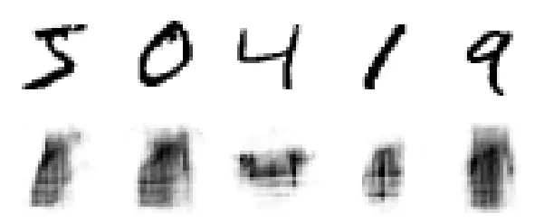

images = mnist_images.to(device)
with torch.no_grad():
    y_pred = stacked_ae(images)
    recon_loss = torch.nn.functional.mse_loss(y_pred, images)

recon_loss # Sai số tái tạo trung bình sẽ rất cao

output:
    tensor(0.0599, device='cuda:0')

Biểu đồ dưới đây so sánh phân phối sai số tái tạo giữa hai tập dữ liệu. Ta thấy rõ sự tách biệt: ảnh MNIST có sai số lớn hơn hẳn, cho phép ta đặt một ngưỡng (threshold) để phát hiện chúng là “bất thường”.

import torch.nn.functional as F

def compute_reconstruction_losses(X, device):
    X = X.to(device)
    with torch.no_grad():
        y_pred = stacked_ae(X)
        # Tính MSE cho từng ảnh, giữ nguyên chiều batch
        return F.mse_loss(y_pred, X, reduction="none").view(X.size(0), -1).mean(dim=1).cpu()

recon_losses_mnist = compute_reconstruction_losses(mnist_images, device)
recon_losses_fashion_mnist = compute_reconstruction_losses(X_valid, device)

plt.hist(recon_losses_mnist, bins=85, alpha=0.8, label="MNIST images")
plt.hist(recon_losses_fashion_mnist, bins=85, alpha=0.8, label="Fashion MNIST images")
plt.xlabel("Reconstruction loss (MSE)")
plt.ylabel("Count", rotation=0)
plt.legend()
plt.grid()

plt.show()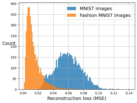

Trực quan hóa Latent Space bằng t-SNE

Chúng ta có thể sử dụng t-SNE để giảm chiều dữ liệu từ không gian mã hóa (32 chiều) xuống 2 chiều để quan sát cách Autoencoder gom cụm các loại quần áo khác nhau.

from sklearn.manifold import TSNE

with torch.no_grad():
    # Lấy vector mã hóa (latent code)
    X_valid_compressed = stacked_encoder(X_valid.to(device))

tsne = TSNE(init="pca", learning_rate="auto", random_state=42)
X_valid_2D = tsne.fit_transform(X_valid_compressed.cpu())

y_valid = torch.tensor([y for _, y in valid_data])

plt.scatter(X_valid_2D[:, 0], X_valid_2D[:, 1], c=y_valid, s=10, cmap="tab10")
plt.show()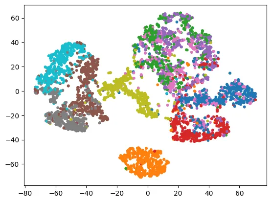

Biểu đồ t-SNE cho thấy các cụm dữ liệu tách biệt khá rõ ràng, chứng tỏ Autoencoder đã học được các đặc trưng ngữ nghĩa (semantic features) có ý nghĩa.

Để biểu đồ đẹp và trực quan hơn (hiển thị cả hình ảnh tại các điểm dữ liệu), ta sử dụng đoạn code sau:

# Code hỗ trợ hiển thị ảnh lên biểu đồ scatter (thẩm mỹ hóa)

import matplotlib as mpl

plt.figure(figsize=(10, 8))
cmap = plt.cm.tab10
Z = X_valid_2D
Z = (Z - Z.min()) / (Z.max() - Z.min())  # Chuẩn hóa về [0, 1]
plt.scatter(Z[:, 0], Z[:, 1], c=y_valid, s=10, cmap=cmap)
image_positions = np.array([[1., 1.]])
for index, position in enumerate(Z):
    dist = ((position - image_positions) ** 2).sum(axis=1)
    if dist.min() > 0.02: # Chỉ vẽ nếu đủ xa các ảnh khác
        image_positions = np.r_[image_positions, [position]]
        imagebox = mpl.offsetbox.AnnotationBbox(
            mpl.offsetbox.OffsetImage(X_valid[index].squeeze(dim=0),
                                      cmap="binary"),
            position, bboxprops={"edgecolor": cmap(y_valid[index]), "lw": 2})
        plt.gca().add_artist(imagebox)

plt.axis("off")

plt.show()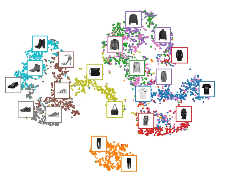

Tying Weights (Ràng buộc trọng số)

Một kỹ thuật phổ biến để giảm số lượng tham số cần huấn luyện và chống overfitting là Tying Weights. Ý tưởng là sử dụng chuyển vị (transpose) của ma trận trọng số Encoder làm trọng số cho Decoder. Nếu Encoder có trọng số $W$, thì Decoder sẽ dùng $W^T$.

Về mặt toán học:

• Encoder: $z = \sigma(W x + b_{enc})$
• Decoder: $\hat{x} = \sigma(W^T z + b_{dec})$

Lưu ý: Bias ($b_{enc}, b_{dec}$) vẫn là các tham số riêng biệt.

import torch.nn.functional as F

class TiedAutoencoder(nn.Module):
    def __init__(self):
        super().__init__()
        self.enc1 = nn.Linear(1 * 28 * 28, 128)
        self.enc2 = nn.Linear(128, 32)
        # Bias Decoder phải được khai báo riêng
        self.dec1_bias = nn.Parameter(torch.zeros(128))
        self.dec2_bias = nn.Parameter(torch.zeros(1 * 28 * 28))

    def encode(self, X):
        Z = X.view(-1, 1 * 28 * 28)  # Flatten
        Z = F.relu(self.enc1(Z))
        return F.relu(self.enc2(Z))

    def decode(self, X):
        # Sử dụng F.linear với trọng số chuyển vị (weight.t())
        Z = F.relu(F.linear(X, self.enc2.weight.t(), self.dec1_bias))
        Z = F.sigmoid(F.linear(Z, self.enc1.weight.t(), self.dec2_bias))
        return Z.view(-1, 1, 28, 28)  # Unflatten

    def forward(self, X):
        return self.decode(self.encode(X))

tied_ae = TiedAutoencoder().to(device)
optimizer = torch.optim.NAdam(tied_ae.parameters(), lr=0.01)
history = train(tied_ae, optimizer, mse, rmse, train_loader, valid_loader, n_epochs=10)

output:
    Epoch 1/10,                      train loss: 0.0229, train metric: 0.151, valid metric: 0.137
    ...
    Epoch 10/10,                      train loss: 0.0124, train metric: 0.112, valid metric: 0.112

# Hiển thị kết quả tái tạo với Tied AE
plot_reconstructions(tied_ae, X_valid)
plt.show()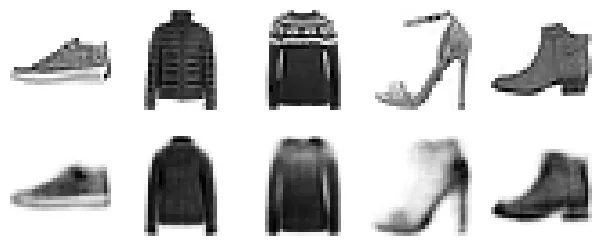

3. Convolutional Autoencoders (CAE)

Đối với dữ liệu hình ảnh, mạng Dense (Linear) không hiệu quả vì nó bỏ qua cấu trúc không gian 2D và tốn quá nhiều tham số. Convolutional Autoencoders giải quyết vấn đề này bằng cách sử dụng các lớp tích chập.

• Encoder: Dùng Conv2d và MaxPool2d để trích xuất đặc trưng và giảm kích thước không gian (spatial dimensions).
• Decoder: Dùng ConvTranspose2d (tích chập chuyển vị) hoặc Upsample kết hợp Conv2d để khôi phục kích thước ảnh.

torch.manual_seed(42)  # Đảm bảo tính tái lập

conv_encoder = nn.Sequential(
    nn.Conv2d(1, 16, kernel_size=3, padding="same"), nn.ReLU(),
    nn.MaxPool2d(kernel_size=2),  # Output: 16 x 14 x 14
    nn.Conv2d(16, 32, kernel_size=3, padding="same"), nn.ReLU(),
    nn.MaxPool2d(kernel_size=2),  # Output: 32 x 7 x 7
    nn.Conv2d(32, 64, kernel_size=3, padding="same"), nn.ReLU(),
    nn.MaxPool2d(kernel_size=2),  # Output: 64 x 3 x 3
    nn.Conv2d(64, 32, kernel_size=3, padding="same"), nn.ReLU(),
    nn.AdaptiveAvgPool2d((1, 1)), nn.Flatten())  # Output: 32 (Latent vector)

conv_decoder = nn.Sequential(
    nn.Linear(32, 16 * 3 * 3),
    nn.Unflatten(dim=1, unflattened_size=(16, 3, 3)),
    # ConvTranspose2d giúp tăng kích thước ảnh (Upsampling)
    nn.ConvTranspose2d(16, 32, kernel_size=3, stride=2), nn.ReLU(),
    nn.ConvTranspose2d(32, 16, kernel_size=3, stride=2, padding=1,
                        output_padding=1), nn.ReLU(),
    nn.ConvTranspose2d(16, 1, kernel_size=3, stride=2, padding=1,
                        output_padding=1), nn.Sigmoid())

conv_ae = nn.Sequential(conv_encoder, conv_decoder).to(device)

optimizer = torch.optim.NAdam(conv_ae.parameters(), lr=0.005)
history = train(conv_ae, optimizer, mse, rmse, train_loader, valid_loader,
                n_epochs=10)

output:
    Epoch 1/10,                      train loss: 0.0297, train metric: 0.172, valid metric: 0.144
    ...
    Epoch 10/10,                      train loss: 0.0120, train metric: 0.11, valid metric: 0.11

# Hiển thị kết quả tái tạo
plot_reconstructions(conv_ae, X_valid)
plt.show()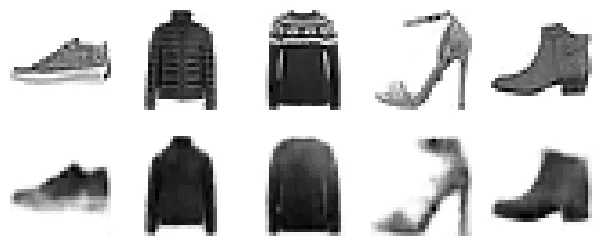

4. Recurrent Autoencoders

Nếu dữ liệu là dạng chuỗi (thời gian, văn bản), ta có thể sử dụng Recurrent Autoencoder với LSTM hoặc GRU. Trong ví dụ này, ta coi mỗi bức ảnh Fashion MNIST như một chuỗi gồm 28 bước (mỗi dòng là một bước thời gian), mỗi bước là một vector 28 chiều.

class RecurrentAutoencoder(nn.Module):
    def __init__(self):
        super().__init__()
        # Encoder dùng LSTM
        self.encoder_lstm = nn.LSTM(input_size=28, hidden_size=128,
                                    num_layers=2, batch_first=True)
        self.encoder_proj = nn.Linear(128, 32)  # Nén hidden state cuối cùng
        # Decoder dùng LSTM
        self.decoder_lstm = nn.LSTM(input_size=32, hidden_size=128,
                                    batch_first=True)
        self.decoder_proj = nn.Linear(128, 28)

    def encode(self, X):  # X shape: [Batch, 1, 28, 28]
        Z = X.squeeze(dim=1)  # Xóa chiều channel -> [Batch, 28, 28]
        _, (h_n, _) = self.encoder_lstm(Z)  # h_n shape: [Num_layers, Batch, Hidden]
        Z = h_n[-1]  # Lấy hidden state của lớp cuối cùng: [Batch, 128]
        return self.encoder_proj(Z)  # [Batch, 32]

    def decode(self, X):
        # Lặp lại latent vector cho mỗi bước thời gian của decoder
        Z = X.unsqueeze(dim=1).repeat(1, 28, 1)  # [Batch, 28, 32]
        Z, _ = self.decoder_lstm(Z)  # [Batch, 28, 128]
        return F.sigmoid(self.decoder_proj(Z).unsqueeze(dim=1)) # [Batch, 1, 28, 28]

    def forward(self, X):
        return self.decode(self.encode(X))

torch.manual_seed(42)
recurrent_ae = RecurrentAutoencoder().to(device)

optimizer = torch.optim.NAdam(recurrent_ae.parameters(), lr=1e-3)
history = train(recurrent_ae, optimizer, mse, rmse, train_loader, valid_loader,
                n_epochs=10)

output:
    Epoch 1/10,                      train loss: 0.0526, train metric: 0.229, valid metric: 0.181
    ...
    Epoch 10/10,                      train loss: 0.0118, train metric: 0.109, valid metric: 0.109

plot_reconstructions(recurrent_ae, X_valid)
plt.show()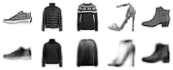

5. Denoising Autoencoders

Lý thuyết

Một Autoencoder thông thường có nguy cơ học thuộc lòng (chỉ sao chép đầu vào ra đầu ra) mà không học được các đặc trưng hữu ích. Denoising Autoencoder giải quyết vấn đề này bằng cách thêm nhiễu vào đầu vào và buộc mạng phải khôi phục lại ảnh gốc không nhiễu.

Mô hình buộc phải học cấu trúc của dữ liệu (Manifold learning) để tách biệt tín hiệu khỏi nhiễu. Input: $\tilde{x} = x + \text{noise}$. Target: $x$. Loss: $L(x, g(f(\tilde{x})))$.

Có hai cách phổ biến để thêm nhiễu:

1. Dropout: Tắt ngẫu nhiên các pixel (gán bằng 0).
2. Gaussian Noise: Cộng thêm nhiễu tuân theo phân phối chuẩn.

Cách 1: Sử dụng Dropout

torch.manual_seed(42)  # Đảm bảo tính tái lập

dropout_encoder = nn.Sequential(
    nn.Flatten(),
    nn.Dropout(0.5), # Tắt 50% pixel ngẫu nhiên
    nn.Linear(1 * 28 * 28, 128), nn.ReLU(),
    nn.Linear(128, 128), nn.ReLU(),
)
dropout_decoder = nn.Sequential(
    nn.Linear(128, 128), nn.ReLU(),
    nn.Linear(128, 1 * 28 * 28), nn.Sigmoid(),
    nn.Unflatten(dim=1, unflattened_size=(1, 28, 28))
)
dropout_ae = nn.Sequential(dropout_encoder, dropout_decoder).to(device)

optimizer = torch.optim.NAdam(dropout_ae.parameters(), lr=0.01)
history = train(dropout_ae, optimizer, mse, rmse, train_loader, valid_loader,
                n_epochs=10)

output:
    Epoch 1/10,                      train loss: 0.0279, train metric: 0.167, valid metric: 0.148
    ...
    Epoch 10/10,                      train loss: 0.0186, train metric: 0.136, valid metric: 0.131

# Hiển thị: Hàng trên là ảnh ĐÃ BỊ NHIỄU, hàng dưới là ảnh TÁI TẠO
torch.manual_seed(42)
dropout = nn.Dropout(0.5)
plot_reconstructions(dropout_ae, dropout(X_valid))

plt.show()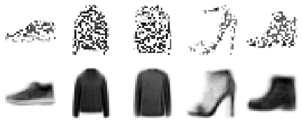

Cách 2: Sử dụng Gaussian Noise

class GaussianNoise(nn.Module):
    def __init__(self, std):
        super().__init__()
        self.std = std

    def forward(self, X):
        if self.training:  # Chỉ thêm nhiễu khi huấn luyện
            noise = torch.randn_like(X) * self.std
            return X + noise
        return X

torch.manual_seed(42)  # Đảm bảo tính tái lập

noise_encoder = nn.Sequential(
    nn.Flatten(),
    GaussianNoise(0.5), # Thêm nhiễu Gaussian
    nn.Linear(1 * 28 * 28, 128), nn.ReLU(),
    nn.Linear(128, 128), nn.ReLU(),
)
noise_decoder = nn.Sequential(
    nn.Linear(128, 128), nn.ReLU(),
    nn.Linear(128, 1 * 28 * 28), nn.Sigmoid(),
    nn.Unflatten(dim=1, unflattened_size=(1, 28, 28))
)
noise_ae = nn.Sequential(noise_encoder, noise_decoder).to(device)

optimizer = torch.optim.NAdam(noise_ae.parameters(), lr=0.01)
history = train(noise_ae, optimizer, mse, rmse, train_loader, valid_loader,
                n_epochs=10)

output:
    Epoch 1/10,                      train loss: 0.0290, train metric: 0.17, valid metric: 0.15
    ...
    Epoch 10/10,                      train loss: 0.0194, train metric: 0.139, valid metric: 0.132

# Hiển thị kết quả khử nhiễu
torch.manual_seed(42)
noise = GaussianNoise(0.5)
plot_reconstructions(noise_ae, noise(X_valid))
plt.show()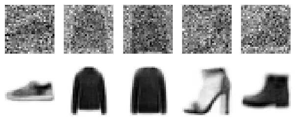

6. Sparse Autoencoder

Lý thuyết

Một cách khác để ràng buộc Autoencoder học các đặc trưng tốt là sử dụng Sparsity Constraint (Ràng buộc thưa). Ta muốn các nơ-ron trong lớp ẩn (coding layer) phần lớn thời gian phải không hoạt động (giá trị gần 0), chỉ một số ít kích hoạt với mỗi mẫu dữ liệu cụ thể.

Ta thêm một thành phần vào hàm mất mát: KL Divergence (Kullback-Leibler Divergence). Nó đo sự khác biệt giữa hai phân phối xác suất:

• $p$: Phân phối thưa mục tiêu (ví dụ: xác suất kích hoạt mong muốn là 0.1).
• $q$: Xác suất kích hoạt trung bình thực tế của nơ-ron trên batch.

Công thức KL Divergence cho hai phân phối Bernoulli: $D_{KL}(p || q) = p \log \frac{p}{q} + (1-p) \log \frac{1-p}{1-q}$

Khi $q$ lệch xa $p$, $D_{KL}$ sẽ tăng cao, buộc mô hình điều chỉnh để $q$ tiến về $p$.

from collections import namedtuple

# Định nghĩa output chứa cả tái tạo và mã hóa để tính loss
AEOutput = namedtuple("AEOutput", ["output", "codings"])

class SparseAutoencoder(nn.Module):
    def __init__(self):
        super().__init__()
        self.encoder = nn.Sequential(
            nn.Flatten(),
            nn.Linear(1 * 28 * 28, 128), nn.ReLU(),
            # Lớp coding dùng Sigmoid để giá trị nằm trong [0, 1]
            nn.Linear(128, 256), nn.Sigmoid())
        self.decoder = nn.Sequential(
            nn.Linear(256, 128), nn.ReLU(),
            nn.Linear(128, 1 * 28 * 28), nn.Sigmoid(),
            nn.Unflatten(dim=1, unflattened_size=(1, 28, 28)))

    def forward(self, X):
        codings = self.encoder(X)
        output = self.decoder(codings)
        return AEOutput(output, codings)

def mse_plus_sparsity_loss(y_pred, y_target, target_sparsity=0.1,
                           kl_weight=1e-3, eps=1e-8):
    p = torch.tensor(target_sparsity, device=y_pred.codings.device)
    # Tính activation trung bình của batch (q)
    q = torch.clamp(y_pred.codings.mean(dim=0), eps, 1 - eps)
    # Công thức KL Divergence
    kl_div = p * torch.log(p / q) + (1 - p) * torch.log((1 - p) / (1 - q))
    # Tổng loss = MSE + KL Divergence Penalty
    return mse(y_pred.output, y_target) + kl_weight * kl_div.sum()

Biểu đồ dưới đây minh họa hàm chi phí KL Divergence. Nó đạt cực tiểu (bằng 0) khi $q = p$ (mức kích hoạt thực tế bằng mức mong muốn).

# Code vẽ đồ thị KL Divergence (Figure 18-10)
plt.figure(figsize=(6, 3.5))
p = 0.1
q = np.linspace(0.001, 0.999, 500)
kl_div = p * np.log(p / q) + (1 - p) * np.log((1 - p) / (1 - q))
mse_ = (p - q) ** 2
mae = np.abs(p - q)
plt.plot([p, p], [0, 0.3], "k:")
plt.text(0.05, 0.32, "Target\nsparsity $p$", fontsize=14)
plt.plot(q, kl_div, "b-", label="KL divergence")
plt.plot(q, mae, "g--", label=r"MAE ($\ell_1$)")
plt.plot(q, mse_, "r--", linewidth=1, label=r"MSE ($\ell_2$)")
plt.legend(loc="upper left", fontsize=14)
plt.xlabel("Actual sparsity $q$")
plt.ylabel("Cost", rotation=0)
plt.axis([0, 1, 0, 0.95])
plt.grid(True)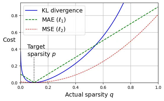

Huấn luyện mô hình với ràng buộc sparsity là 10%.

torch.manual_seed(42)
sparse_ae = SparseAutoencoder().to(device)
optimizer = torch.optim.NAdam(sparse_ae.parameters(), lr=0.002)
history = train(sparse_ae, optimizer, mse_plus_sparsity_loss, rmse,
                train_loader, valid_loader, n_epochs=10)

output:
    Epoch 1/10,                      train loss: 0.0288, train metric: 0.166, valid metric: 0.134
    ...
    Epoch 10/10,                      train loss: 0.0085, train metric: 0.0906, valid metric: 0.0911

# Hiển thị kết quả tái tạo
plot_reconstructions(sparse_ae, X_valid)
plt.show()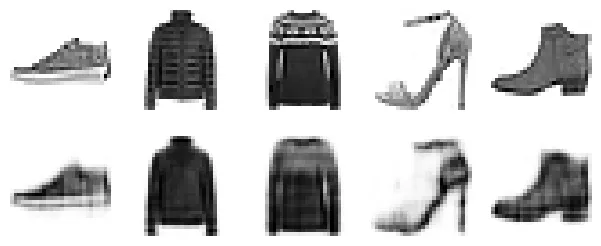

Kiểm tra xem mô hình có thực sự “thưa” không bằng cách vẽ biểu đồ histogram các giá trị kích hoạt.

with torch.no_grad():
    y_pred = sparse_ae(X_valid.to(device))

encs = y_pred.codings.flatten().detach().cpu()
plt.hist(encs, log=True)
plt.xlabel("Activation")
plt.ylabel("Count")
plt.show()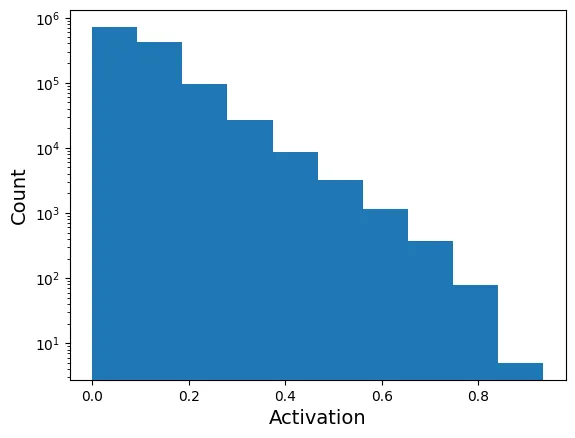

# Giá trị kích hoạt trung bình (nên gần 0.1)
y_pred.codings.mean()

output:
    tensor(0.1016, device='cuda:0')

Một tính chất thú vị của Sparse AE là các nơ-ron thường chuyên biệt hóa. Ví dụ, ta có thể tìm xem những ảnh nào kích hoạt mạnh nơ-ron số 6.

def plot_multiple_images(images, n_cols=None):
    n_cols = n_cols or len(images)
    n_rows = (len(images) - 1) // n_cols + 1
    plt.figure(figsize=(n_cols, n_rows))
    for index, image in enumerate(images):
        plt.subplot(n_rows, n_cols, index + 1)
        plot_image(image)

dim = 6
codings = y_pred.codings[:, dim].cpu()
threshold = np.percentile(codings, 90)
# Chọn các ảnh có activation > 90th percentile tại dim 6
selected_images = X_valid[codings > threshold]
plot_multiple_images(selected_images[:35], 7)
plt.show()

7. Variational Autoencoder (VAE)

Lý thuyết nền tảng

Variational Autoencoder (VAE) là một bước nhảy vọt quan trọng. Khác với AE truyền thống ánh xạ đầu vào thành một vector cố định, VAE ánh xạ đầu vào thành một phân phối xác suất (thường là phân phối chuẩn Gaussian).

Mô hình giả định dữ liệu được sinh ra từ một biến tiềm ẩn $z$. Encoder sẽ dự đoán hai tham số của phân phối:

1. Mean (Trung bình) $\mu$
2. Log Variance (Log phương sai) $\log(\sigma^2)$

Từ đó ta lấy mẫu (sample) $z$ từ phân phối này và đưa vào Decoder.

Reparameterization Trick (Thủ thuật tái tham số hóa): Việc lấy mẫu $z \sim \mathcal{N}(\mu, \sigma^2)$ là ngẫu nhiên và không thể lan truyền ngược (backpropagation). Do đó, ta sử dụng công thức: $z = \mu + \sigma \odot \epsilon$ trong đó $\epsilon \sim \mathcal{N}(0, I)$. Lúc này tính ngẫu nhiên nằm ở $\epsilon$ (hằng số đối với gradient), cho phép gradient đi qua $\mu$ và $\sigma$.

Hàm mất mát (ELBO - Evidence Lower Bound): $Loss = \text{Reconstruction Loss} + \text{KL Divergence Loss}$

• Thành phần tái tạo: Đảm bảo ảnh đầu ra giống đầu vào.
• Thành phần KL: Đảm bảo phân phối tiềm ẩn gần với phân phối chuẩn tắc $\mathcal{N}(0, I)$, giúp không gian tiềm ẩn liên tục và mượt mà, thuận lợi cho việc sinh dữ liệu mới.

VAEOutput = namedtuple("VAEOutput",
                       ["output", "codings_mean", "codings_logvar"])

class VAE(nn.Module):
    def __init__(self, codings_dim=32):
        super(VAE, self).__init__()
        self.codings_dim = codings_dim
        self.encoder = nn.Sequential(
            nn.Flatten(),
            nn.Linear(1 * 28 * 28, 128), nn.ReLU(),
            # Output kích thước 2 * codings_dim để chứa cả mean và logvar
            nn.Linear(128, 2 * codings_dim))
        self.decoder = nn.Sequential(
            nn.Linear(codings_dim, 128), nn.ReLU(),
            nn.Linear(128, 1 * 28 * 28), nn.Sigmoid(),
            nn.Unflatten(dim=1, unflattened_size=(1, 28, 28)))

    def encode(self, X):
        # Chia output thành 2 phần: mean và logvar
        return self.encoder(X).chunk(2, dim=-1)

    def sample_codings(self, codings_mean, codings_logvar):
        codings_std = torch.exp(0.5 * codings_logvar)
        noise = torch.randn_like(codings_std) # Epsilon ~ N(0, I)
        return codings_mean + noise * codings_std # Reparameterization trick

    def decode(self, Z):
        return self.decoder(Z)

    def forward(self, X):
        codings_mean, codings_logvar = self.encode(X)
        codings = self.sample_codings(codings_mean, codings_logvar)
        output = self.decode(codings)
        return VAEOutput(output, codings_mean, codings_logvar)

def vae_loss(y_pred, y_target, kl_weight=1.0):
    output, mean, logvar = y_pred
    # Công thức KL Divergence giữa N(mean, std) và N(0, 1)
    kl_div = -0.5 * torch.sum(1 + logvar - logvar.exp() - mean.square(), dim=-1)
    # Tổng hợp loss: MSE + KL (được chuẩn hóa theo số pixel)
    return F.mse_loss(output, y_target) + kl_weight * kl_div.mean() / 784

torch.manual_seed(42)
vae = VAE().to(device)
optimizer = torch.optim.NAdam(vae.parameters(), lr=1e-3)
history = train(vae, optimizer, vae_loss, rmse, train_loader, valid_loader,
                n_epochs=20)

output:
    Epoch 1/20,                      train loss: 0.0491, train metric: 0.199, valid metric: 0.174
    ...
    Epoch 20/20,                      train loss: 0.0318, train metric: 0.147, valid metric: 0.148

plot_reconstructions(vae, X_valid)
plt.show()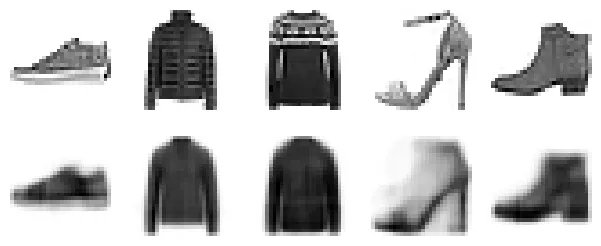

Sinh ảnh mới (Generative)

Bởi vì VAE ép buộc latent space phải tuân theo phân phối chuẩn $\mathcal{N}(0, I)$, ta có thể sinh ra ảnh mới hoàn toàn bằng cách lấy mẫu ngẫu nhiên $z \sim \mathcal{N}(0, I)$ và đưa vào Decoder.

torch.manual_seed(42)  # Đảm bảo tính tái lập

vae.eval()
# Lấy mẫu ngẫu nhiên từ phân phối chuẩn
codings = torch.randn(3 * 7, vae.codings_dim, device=device)
with torch.no_grad():
    images = vae.decode(codings)

# Hiển thị ảnh sinh ra từ nhiễu
plot_multiple_images(images, 7)
plt.show()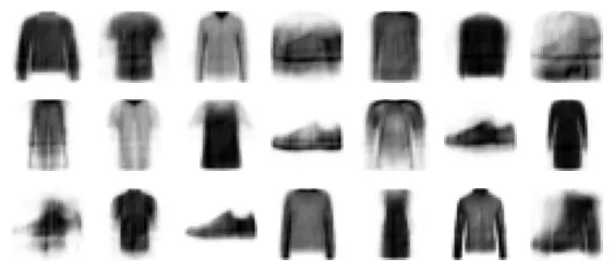

Nội suy ngữ nghĩa (Semantic Interpolation)

Một đặc điểm tuyệt vời của VAE là không gian tiềm ẩn rất “mượt”. Nếu ta lấy hai điểm $z_1, z_2$ đại diện cho hai ảnh và di chuyển từ từ từ $z_1$ sang $z_2$, các ảnh giải mã được sẽ biến đổi hình thái (morphing) một cách liên tục, không bị gãy khúc hay ra nhiễu.

torch.manual_seed(111)  # Đảm bảo tính tái lập

codings = torch.randn(2, vae.codings_dim)  # Điểm đầu và điểm cuối
n_images = 7
weights = torch.linspace(0, 1, n_images).view(n_images, 1)
# Nội suy tuyến tính (Linear Interpolation)
codings = torch.lerp(codings[0], codings[1], weights)
with torch.no_grad():
    images = vae.decode(codings.to(device))

plot_multiple_images(images)
plt.show()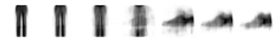

8. Discrete VAE (DALL-E’s ancestor)

Một số mô hình hiện đại (như DALL-E đời đầu hay VQ-VAE) sử dụng không gian tiềm ẩn rời rạc (discrete) thay vì liên tục. Để huấn luyện được với backpropagation trên dữ liệu rời rạc, chúng ta sử dụng Gumbel-Softmax trick.

Lưu ý kỹ thuật: Hiện tại có một lỗi trong F.gumbel_softmax trên thiết bị MPS (Apple Silicon). Đoạn code dưới đây bao gồm bản vá lỗi (workaround) để đảm bảo chạy ổn định trên mọi thiết bị.

def gumbel_softmax(logits, tau=1, hard=False, dim=-1):
    if device != "mps":
        return F.gumbel_softmax(logits, tau, hard, dim)

    # Triển khai thủ công cho MPS để tránh bug
    gumbels = (
        -torch.empty_like(logits, memory_format=torch.legacy_contiguous_format)
        .exponential_()
        .log()
    )  # Tạo nhiễu Gumbel ~Gumbel(0,1)
    gumbels = torch.clamp(gumbels, -30, 30)  # Giới hạn giá trị để tránh NaN
    gumbels = (logits + gumbels) / tau  # ~Gumbel(logits, tau)
    y_soft = gumbels.softmax(dim)

    if hard:
        # Straight through estimator: Forward là one-hot, Backward là soft gradient
        index = y_soft.max(dim, keepdim=True)[1]
        y_hard = torch.zeros_like(
            logits, memory_format=torch.legacy_contiguous_format
        ).scatter_(dim, index, 1.0)
        ret = y_hard - y_soft.detach() + y_soft
    else:
        # Reparametrization trick thường
        ret = y_soft
    return ret

DiscreteVAEOutput = namedtuple("DiscreteVAEOutput",
                               ["output", "logits", "codings_prob"])

class DiscreteVAE(nn.Module):
    def __init__(self, coding_length=32, n_codes=16, temperature=1.0):
        super().__init__()
        self.coding_length = coding_length
        self.n_codes = n_codes
        self.temperature = temperature
        self.encoder = nn.Sequential(
            nn.Flatten(),
            nn.Linear(1 * 28 * 28, 256), nn.ReLU(),
            nn.Linear(256, 128), nn.ReLU(),
            nn.Linear(128, coding_length * n_codes),
            nn.Unflatten(dim=1, unflattened_size=(coding_length, n_codes)))
        self.decoder = nn.Sequential(
            nn.Flatten(),
            nn.Linear(coding_length * n_codes, 128), nn.ReLU(),
            nn.Linear(128, 256), nn.ReLU(),
            nn.Linear(256, 1 * 28 * 28), nn.Sigmoid(),
            nn.Unflatten(dim=1, unflattened_size=(1, 28, 28)))

    def forward(self, X):
        logits = self.encoder(X)
        # Sử dụng Gumbel-Softmax để lấy mẫu rời rạc nhưng vẫn khả vi
        codings_prob = gumbel_softmax(logits, tau=self.temperature, hard=True)
        output = self.decoder(codings_prob)
        return DiscreteVAEOutput(output, logits, codings_prob)

def d_vae_loss(y_pred, y_target, kl_weight=1.0):
    output, logits, _ = y_pred
    codings_prob = F.softmax(logits, -1)
    # Tính KL Divergence so với phân phối đều (Uniform distribution)
    k = logits.new_tensor(logits.size(-1))
    kl_div = (codings_prob * (codings_prob.log() + k.log())).sum(dim=(1, 2))
    return F.mse_loss(output, y_target) + kl_weight * kl_div.mean() / 784

n_epochs = 20
# Giảm dần nhiệt độ (temperature annealing) giúp mô hình hội tụ về rời rạc cứng
def annealing(model, epoch):
    model.temperature = 1 - 0.9 * epoch / n_epochs

torch.manual_seed(42)
d_vae = DiscreteVAE().to(device)
optimizer = torch.optim.NAdam(d_vae.parameters(), lr=0.001)
history = train(d_vae, optimizer, d_vae_loss, rmse, train_loader, valid_loader,
                n_epochs=n_epochs, epoch_callback=annealing)

output:
    Epoch 1/20,                      train loss: 0.0580, train metric: 0.228, valid metric: 0.209
    ...
    Epoch 20/20,                      train loss: 0.0361, train metric: 0.167, valid metric: 0.168

torch.manual_seed(42)  # Đảm bảo tính tái lập
n_images = 3 * 7
# Sinh mã ngẫu nhiên từ 0 đến k-1
codings = torch.randint(0, d_vae.n_codes,
                        (n_images, d_vae.coding_length), device=device)
codings_prob = F.one_hot(codings, num_classes=d_vae.n_codes).float()
with torch.no_grad():
    images = d_vae.decoder(codings_prob)

plot_multiple_images(images, 7)
plt.show()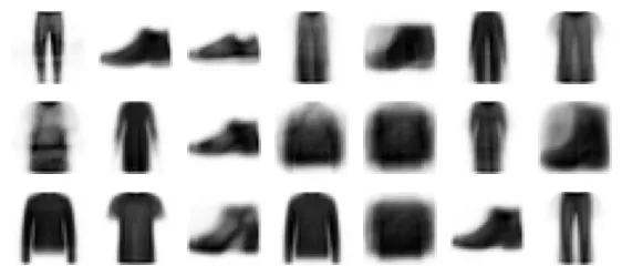

9. Generative Adversarial Networks (GANs)

Lý thuyết nền tảng

Được đề xuất bởi Ian Goodfellow năm 2014, GANs là một cuộc chơi đối kháng giữa hai mạng:

1. Generator (G - Kẻ làm giả): Nhận đầu vào là nhiễu ngẫu nhiên $z$ và cố gắng tạo ra ảnh giả $G(z)$ giống thật nhất có thể để đánh lừa Discriminator.
2. Discriminator (D - Cảnh sát): Nhận đầu vào là ảnh (cả thật $x$ và giả $G(z)$) và cố gắng phân loại xem đó là ảnh thật hay giả.

Mục tiêu là đạt đến Nash Equilibrium (Cân bằng Nash), nơi Generator tạo ra ảnh hoàn hảo đến mức Discriminator chỉ có thể đoán ngẫu nhiên (xác suất 0.5).

Hàm giá trị (Value function) của trò chơi Minimax này: $\min_G \max_D V(D, G) = \mathbb{E}_{x \sim p_{data}(x)}[\log D(x)] + \mathbb{E}_{z \sim p_z(z)}[\log(1 - D(G(z)))]$

torch.manual_seed(42)  # Đảm bảo tính tái lập

codings_dim = 32
# Generator: Noise -> Image
generator = nn.Sequential(
    nn.Linear(codings_dim, 128), nn.ReLU(),
    nn.Linear(128, 256), nn.ReLU(),
    nn.Linear(256, 1 * 28 * 28), nn.Sigmoid(),
    nn.Unflatten(dim=1, unflattened_size=(1, 28, 28))).to(device)

# Discriminator: Image -> Probability (Real/Fake)
discriminator = nn.Sequential(
    nn.Flatten(),
    nn.Linear(1 * 28 * 28, 256), nn.ReLU(),
    nn.Linear(256, 128), nn.ReLU(),
    nn.Linear(128, 1), nn.Sigmoid()).to(device)

Quá trình huấn luyện GAN rất khó khăn và không ổn định. Chúng ta cần huấn luyện xen kẽ: train D một bước, rồi train G một bước. Lưu ý quan trọng: khi train G, ta phải đóng băng trọng số của D.

def train_gan(generator, discriminator, train_loader, codings_dim, n_epochs=20,
              g_lr=1e-3, d_lr=5e-4):
    criterion = nn.BCELoss()
    generator_opt = torch.optim.NAdam(generator.parameters(), lr=g_lr)
    discriminator_opt = torch.optim.NAdam(discriminator.parameters(), lr=d_lr)

    for epoch in range(n_epochs):
        print(f"Epoch {epoch + 1}/{n_epochs}", end="")
        for real_images, _ in train_loader:
            real_images = real_images.to(device)
            batch_size = real_images.size(0)

            # --- Giai đoạn 1: Huấn luyện Discriminator ---
            # D đoán ảnh thật
            pred_real = discriminator(real_images)
            ones = torch.ones(batch_size, 1, device=device)
            real_loss = criterion(pred_real, ones)

            # D đoán ảnh giả (được sinh từ G)
            codings = torch.randn(batch_size, codings_dim, device=device)
            fake_images = generator(codings).detach() # Detach để không tính grad cho G
            pred_fake = discriminator(fake_images)
            zeros = torch.zeros(batch_size, 1, device=device)
            fake_loss = criterion(pred_fake, zeros)

            # Tổng hợp loss cho D và cập nhật
            discriminator_loss = real_loss + fake_loss
            discriminator_opt.zero_grad()
            discriminator_loss.backward()
            discriminator_opt.step()

            # --- Giai đoạn 2: Huấn luyện Generator ---
            codings = torch.randn(batch_size, codings_dim, device=device)
            fake_images = generator(codings)
            # Đóng băng D tạm thời (chỉ cập nhật G)
            for p in discriminator.parameters():
                p.requires_grad = False
            pred_fake = discriminator(fake_images)
            # G muốn đánh lừa D -> Target là 1 (Real)
            generator_loss = criterion(pred_fake, ones)
            generator_opt.zero_grad()
            generator_loss.backward()
            generator_opt.step()
            # Mở khóa D
            for p in discriminator.parameters():
                p.requires_grad = True

        print(f" | discriminator loss: {discriminator_loss.item():.4f}", end="")
        print(f" | generator loss: {generator_loss.item():.4f}")
        if epoch % 10 == 0 or epoch == n_epochs - 1:
            plot_multiple_images(fake_images.detach(), 8)
            plt.show()

torch.manual_seed(41)  # Đổi seed đôi khi giúp tránh hội tụ xấu
train_gan(generator, discriminator, train_loader, codings_dim)

output:
    Epoch 1/20 | discriminator loss: 0.9104 | generator loss: 7.2512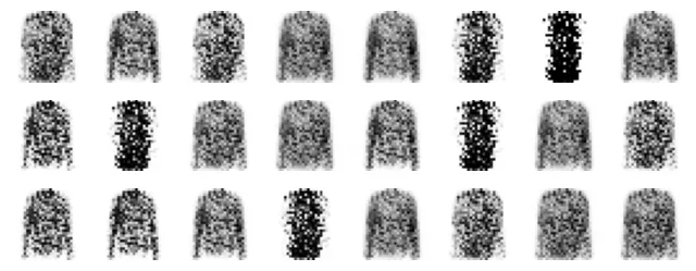

output:
    ...
    Epoch 11/20 | discriminator loss: 1.4950 | generator loss: 2.4509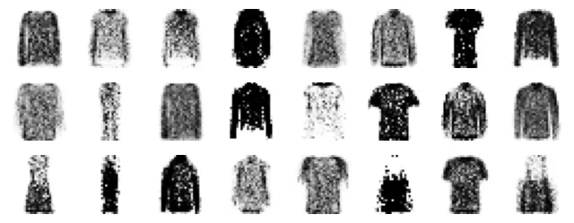

output:
    ...
    Epoch 20/20 | discriminator loss: 0.8947 | generator loss: 1.6881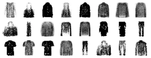

Deep Convolutional GAN (DCGAN)

Để tạo ảnh tốt hơn, chúng ta sử dụng kiến trúc tích chập sâu (DCGAN). Các nguyên tắc chính:

• Thay Pooling bằng Strided Convolutions (Discriminator) và Fractional-Strided Convolutions (Generator).
• Sử dụng Batch Normalization.
• Dùng ReLU/LeakyReLU cho các lớp ẩn, và Tanh cho lớp output của Generator.

torch.manual_seed(1)  # Đảm bảo tính tái lập

dc_codings_dim = 100

dc_generator = nn.Sequential(
    nn.Linear(dc_codings_dim, 128 * 7 * 7),
    nn.Unflatten(dim=1, unflattened_size=(128, 7, 7)),
    nn.BatchNorm2d(128),
    nn.ConvTranspose2d(128, 64, kernel_size=3, stride=2, padding=1,
                       output_padding=1), nn.ReLU(),
    nn.BatchNorm2d(64),
    nn.ConvTranspose2d(64, 1, kernel_size=3, stride=2, padding=1,
                       output_padding=1), nn.Sigmoid()).to(device)

dc_discriminator = nn.Sequential(
    nn.Conv2d(1, 32, kernel_size=5, stride=2, padding=2), nn.ReLU(),  # 32 x 14 x 14
    nn.Dropout(0.4),
    nn.Conv2d(32, 64, kernel_size=5, stride=2, padding=2), nn.ReLU(),  # 64 x 7 x 7
    nn.Dropout(0.4),
    nn.Flatten(),
    nn.Linear(64 * 7 * 7, 1), nn.Sigmoid()).to(device)

torch.manual_seed(42)
train_gan(dc_generator, dc_discriminator, train_loader, dc_codings_dim)

output:
    Epoch 1/20 | discriminator loss: 1.3175 | generator loss: 0.7800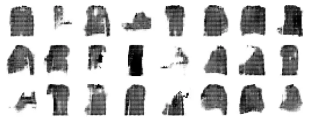

output:
    ...
    Epoch 11/20 | discriminator loss: 0.5970 | generator loss: 1.5689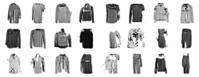

output:
    ...
    Epoch 20/20 | discriminator loss: 0.6701 | generator loss: 1.7119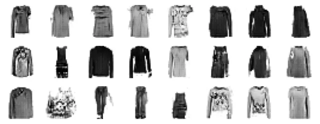

10. Diffusion Models (Mô hình khuếch tán)

Lý thuyết và Cơ sở Toán học

Diffusion Models lấy cảm hứng từ nhiệt động lực học không cân bằng. Ý tưởng cốt lõi bao gồm hai quá trình:

1. Forward Process (Quá trình khuếch tán): Phá hủy cấu trúc dữ liệu bằng cách thêm dần nhiễu Gaussian qua $T$ bước thời gian. Tại bước $T$, dữ liệu trở thành nhiễu trắng thuần túy. $q(x_t | x_{t-1}) = \mathcal{N}(x_t; \sqrt{1-\beta_t}x_{t-1}, \beta_t \mathbf{I})$ Nhờ tính chất của phân phối Gauss, ta có thể nhảy cóc từ $x_0$ đến $x_t$ bất kỳ: $x_t = \sqrt{\bar{\alpha}_t} x_0 + \sqrt{1 - \bar{\alpha}_t} \epsilon$ Với $\alpha_t = 1 - \beta_t$ và $\bar{\alpha}_t = \prod_{s=1}^t \alpha_s$.

2. Reverse Process (Quá trình khử nhiễu): Huấn luyện một mạng nơ-ron để đảo ngược quá trình trên, tức là dự đoán $x_{t-1}$ từ $x_t$. Thực chất, mô hình học cách dự đoán lượng nhiễu $\epsilon$ đã được thêm vào.

Dưới đây, chúng ta cài đặt lịch trình phương sai (Variance Schedule) sử dụng hàm cosine (theo bài báo Improved DDPM) để kiểm soát lượng nhiễu thêm vào.

def variance_schedule(T, s=0.008, max_beta=0.999):
    t = torch.linspace(0, T, T + 1)
    # Sử dụng lịch trình cosine thay vì tuyến tính để ổn định hơn
    f = torch.cos((t / T + s) / (1 + s) * torch.pi / 2) ** 2
    alpha_bars = f / f[0]
    betas = (1 - (f[1:] / f[:-1])).clamp(max=max_beta)
    betas = torch.cat([torch.zeros(1), betas])  # Thêm 0 vào đầu để dễ index
    alphas = 1 - betas
    return alphas, betas, alpha_bars

torch.manual_seed(42)
T = 4000 # Tổng số bước thời gian
alphas, betas, alpha_bars = variance_schedule(T)

Biểu đồ dưới đây cho thấy sự thay đổi của $\beta_t$ (lượng nhiễu thêm vào mỗi bước) và $\bar{\alpha}_t$ (lượng thông tin gốc còn giữ lại) theo thời gian.

# Vẽ đồ thị lịch trình phương sai (Figure 18-21)
plt.figure(figsize=(6, 3))
plt.plot(betas, "r--", label=r"$\beta_t$")
plt.plot(alpha_bars, "b", label=r"$\bar{\alpha}_t$")
plt.axis([0, T, 0, 1.01])
plt.grid(True)
plt.xlabel("$t$")
plt.ylabel(r"Value")
plt.legend()

plt.show()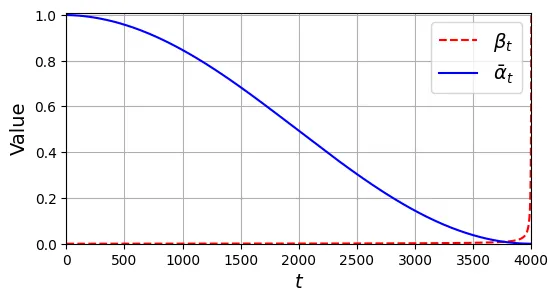

Hàm forward_diffusion thực hiện công thức nhảy cóc để tạo ra ảnh nhiễu tại bước $t$ từ ảnh gốc $x_0$.

def forward_diffusion(x0, t):
    eps = torch.randn_like(x0)  # Nhiễu mục tiêu (Target Noise)
    # Công thức x_t = sqrt(alpha_bar) * x0 + sqrt(1 - alpha_bar) * eps
    xt = alpha_bars[t].sqrt() * x0 + (1 - alpha_bars[t]).sqrt() * eps
    return xt, eps

Định nghĩa cấu trúc dữ liệu đầu vào cho mô hình.

from collections import namedtuple

class DiffusionSample(namedtuple("DiffusionSampleBase", ["xt", "t"])):
    def to(self, device):
        return DiffusionSample(self.xt.to(device), self.t.to(device))

Chúng ta cần một Dataset Wrapper để thực hiện quá trình thêm nhiễu (Forward Diffusion) ngay trong lúc lấy dữ liệu (on-the-fly). Mỗi lần lấy, mô hình sẽ nhận một ảnh đã bị thêm nhiễu ở thời điểm $t$ ngẫu nhiên và nhiệm vụ là dự đoán lớp nhiễu eps đó.

class DiffusionDataset:
    def __init__(self, dataset):
        self.dataset = dataset

    def __getitem__(self, i):
        x0, _ = self.dataset[i]
        x0 = (x0 * 2) - 1  # Chuẩn hóa về [-1, 1]
        t = torch.randint(1, T + 1, size=[1]) # Chọn ngẫu nhiên bước thời gian t
        xt, eps = forward_diffusion(x0, t)
        return DiffusionSample(xt, t), eps

    def __len__(self):
        return len(self.dataset)

train_set = DiffusionDataset(train_data)
train_loader = DataLoader(train_set, batch_size=32, shuffle=True)
valid_set = DiffusionDataset(valid_data)
valid_loader = DataLoader(valid_set, batch_size=32)

Kiểm tra nhanh dữ liệu: Ảnh gốc, Ảnh nhiễu (Input), và Nhiễu cần dự đoán (Target).

# Hàm hỗ trợ khôi phục ảnh gốc từ ảnh nhiễu và nhiễu (để kiểm tra công thức)
def original_image(sample, noise):
    alpha_bars_t = torch.gather(alpha_bars, dim=0, index=sample.t.squeeze(1))
    alpha_bars_t = alpha_bars_t.view(-1, 1, 1, 1)
    x0 = (sample.xt - (1 - alpha_bars_t).sqrt() * noise) / alpha_bars_t.sqrt()
    return torch.clamp((x0 + 1) / 2, 0, 1)

torch.manual_seed(42)
sample, eps = next(iter(train_loader))
x0 = original_image(sample, eps).to(device)

print("Original images")
plot_multiple_images(x0[:8])
plt.show()
print("Time steps:", sample.t[:8].view(-1).tolist())
print("Noisy images")
plot_multiple_images(sample.xt[:8])
plt.show()
print("Noise to predict")
plot_multiple_images(eps[:8])
plt.show()

output:
    Original images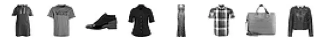

output:
    Time steps: [2027, 1463, 3720, 9, 611, 2202, 2118, 388]
    Noisy images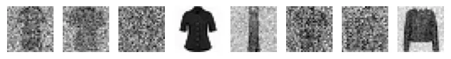

output:
    Noise to predict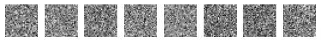

Kiến trúc Mạng: UNet với Time Embedding

Mô hình cần biết nó đang ở bước thời gian $t$ nào để quyết định mức độ khử nhiễu. Do đó, ta cần Time Encoding (tương tự Positional Encoding trong Transformer). Ta sử dụng hàm Sinusoidal.

embed_dim = 64

class TimeEncoding(nn.Module):
    def __init__(self, T, embed_dim):
        super().__init__()
        assert embed_dim % 2 == 0, "embed_dim must be even"
        p = torch.arange(T + 1).unsqueeze(1)
        # Tính toán encoding dựa trên tần số sin/cos
        angle = p / 10_000 ** (torch.arange(0, embed_dim, 2) / embed_dim)
        te = torch.empty(T + 1, embed_dim)
        te[:, 0::2] = torch.sin(angle)
        te[:, 1::2] = torch.cos(angle)
        self.register_buffer("time_encodings", te)

    def forward(self, t):
        return self.time_encodings[t]

Chúng ta xây dựng mạng UNet - kiến trúc tiêu chuẩn cho Diffusion Models. Nó có cấu trúc đối xứng hình chữ U:

• Down path: Giảm kích thước không gian, tăng số kênh.
• Up path: Tăng kích thước không gian, giảm số kênh, kết hợp với Skip Connections từ Down path.
• Time Adapter: Nhúng thông tin thời gian $t$ vào từng khối của mạng (thường là cộng vào feature map).

class SeparableConv2d(nn.Module):
    def __init__(self, in_channels, out_channels, kernel_size, padding):
        super().__init__()
        # Depthwise Conv: Tích chập riêng cho từng kênh
        self.depthwise = nn.Conv2d(in_channels, in_channels, kernel_size,
                                   padding=padding, groups=in_channels)
        # Pointwise Conv: Trộn các kênh lại (1x1 conv)
        self.pointwise = nn.Conv2d(in_channels, out_channels, kernel_size=1)

    def forward(self, X):
        return self.pointwise(self.depthwise(X))

class DiffusionModel(nn.Module):
    def __init__(self, T=T, embed_dim=64):
        super().__init__()
        self.time_encoding = TimeEncoding(T, embed_dim)

        # Init Block
        dim = 16
        self.pad = nn.ConstantPad2d((3, 3, 3, 3), 0)
        self.init_conv = nn.Conv2d(1, dim, kernel_size=3)
        self.init_bn = nn.BatchNorm2d(dim)
        self.time_adapter_init = nn.Linear(embed_dim, dim)

        # Down path (Encoder)
        self.down_blocks = nn.ModuleList()
        self.skip_convs = nn.ModuleList()
        self.time_adapters_down = nn.ModuleList()
        in_dim = dim
        for dim in (32, 64, 128):
            block = nn.Sequential(
                nn.ReLU(),
                SeparableConv2d(in_dim, dim, kernel_size=3, padding=1),
                nn.BatchNorm2d(dim),
                nn.ReLU(),
                SeparableConv2d(dim, dim, kernel_size=3, padding=1),
                nn.BatchNorm2d(dim)
            )
            skip_conv = nn.Conv2d(in_dim, dim, kernel_size=1, stride=2)
            self.down_blocks.append(block)
            self.skip_convs.append(skip_conv)
            self.time_adapters_down.append(nn.Linear(embed_dim, dim))
            in_dim = dim

        # Up path (Decoder)
        self.up_blocks = nn.ModuleList()
        self.skip_up_convs = nn.ModuleList()
        self.time_adapters_up = nn.ModuleList()
        for dim in (64, 32, 16):
            block = nn.Sequential(
                nn.ReLU(),
                # ConvTranspose2d để tăng kích thước
                nn.ConvTranspose2d(in_dim, dim, 3, padding=1),
                nn.BatchNorm2d(dim),
                nn.ReLU(),
                nn.ConvTranspose2d(dim, dim, 3, padding=1),
                nn.BatchNorm2d(dim)
            )
            skip_conv = nn.Conv2d(in_dim, dim, kernel_size=1)
            self.up_blocks.append(block)
            self.skip_up_convs.append(skip_conv)
            self.time_adapters_up.append(nn.Linear(embed_dim, dim))
            in_dim = dim * 3  # *3 vì nối (concatenate) với skip connection

        self.final_conv = nn.Conv2d(in_dim, 1, 3, padding=1)

    def forward(self, sample):
        if not isinstance(sample, DiffusionSample):
            print(repr(sample))
        # Mã hóa thời gian
        time_enc = self.time_encoding(sample.t.squeeze(1))  # [batch, embed_dim]
        z = self.pad(sample.xt)
        z = F.relu(self.init_bn(self.init_conv(z)))
        # Cộng thông tin thời gian vào feature map
        z = z + self.time_adapter_init(time_enc)[:, :, None, None]
        skip = z
        cross_skips = []

        # Downsampling path
        for block, skip_conv, time_adapter in zip(
                self.down_blocks, self.skip_convs, self.time_adapters_down):
            z = block(z)
            cross_skips.append(z)
            z = F.max_pool2d(z, 3, stride=2, padding=1)
            skip_link = skip_conv(skip)
            z = z + skip_link
            z = z + time_adapter(time_enc)[:, :, None, None]
            skip = z

        # Upsampling path
        for block, skip_up_conv, time_adapter in zip(
                self.up_blocks, self.skip_up_convs, self.time_adapters_up):
            z = block(z)
            z = F.interpolate(z, scale_factor=2, mode="nearest")
            skip_link = F.interpolate(skip, scale_factor=2, mode="nearest")
            skip_link = skip_up_conv(skip_link)
            z = z + skip_link
            z = z + time_adapter(time_enc)[:, :, None, None]
            cross_skip = cross_skips.pop()
            # Nối feature map hiện tại với feature map từ Encoder (Skip connection)
            z = torch.cat([z, cross_skip], dim=1)
            skip = z

        out = self.final_conv(z)
        out = out[:, :, 2:-2, 2:-2]  # Cắt bỏ phần padding thừa
        return out.contiguous()

Tiến hành huấn luyện. Chúng ta sử dụng Huber Loss thay vì MSE vì nó ít nhạy cảm hơn với các ngoại lai (outliers) và ổn định hơn khi huấn luyện Diffusion.

torch.manual_seed(42)
diffusion_model = DiffusionModel().to(device)
huber = nn.HuberLoss()
optimizer = torch.optim.NAdam(diffusion_model.parameters(), lr=3e-3)
rmse = torchmetrics.MeanSquaredError(squared=False).to(device)

history = train(diffusion_model, optimizer, huber, rmse, train_loader,
                valid_loader, n_epochs=20)

output:
    Epoch 1/20,                      train loss: 0.0780, train metric: 0.449, valid metric: 0.334
    ...
    Epoch 20/20,                      train loss: 0.0388, train metric: 0.288, valid metric: 0.285

Sinh ảnh với DDPM (Denoising Diffusion Probabilistic Models)

Để sinh ảnh, ta bắt đầu từ nhiễu trắng $x_T \sim \mathcal{N}(0, I)$ và thực hiện ngược lại quá trình khuếch tán. Tại mỗi bước $t$, mô hình dự đoán nhiễu $\epsilon_\theta(x_t, t)$, sau đó ta trừ bớt một phần nhiễu này để thu được $x_{t-1}$. Quá trình lặp lại cho đến khi về $x_0$.

def generate_ddpm(model, batch_size=32):
    model.eval()
    with torch.no_grad():
        # Bắt đầu từ nhiễu trắng tại t=T
        xt = torch.randn([batch_size, 1, 28, 28], device=device)
        for t in range(T, 0, -1):
            print(f"\rt = {t}", end=" ")  # In tiến độ
            alpha_t = alphas[t]
            beta_t = betas[t]
            alpha_bar_t = alpha_bars[t]

            # Thêm nhiễu ngẫu nhiên z vào quá trình lấy mẫu (trừ bước cuối cùng)
            noise = (torch.randn(xt.shape, device=device)
                     if t > 1 else torch.zeros(xt.shape, device=device))
            t_batch = torch.full((batch_size, 1), t, device=device)
            sample = DiffusionSample(xt, t_batch)

            # Dự đoán nhiễu
            eps_pred = model(sample)

            # Công thức cập nhật x_{t-1} (Algorithm 2 trong bài báo DDPM)
            xt = (1 / alpha_t.sqrt()
                  * (xt - beta_t / (1 - alpha_bar_t).sqrt() * eps_pred)
                  + (1 - alpha_t).sqrt() * noise)
        return torch.clamp((xt + 1) / 2, 0, 1)

torch.manual_seed(42)
X_gen = generate_ddpm(diffusion_model)

output:
    t = 1 

plot_multiple_images(X_gen, 8)
plt.show()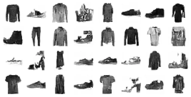

Chất lượng ảnh sinh ra rất ấn tượng và đa dạng. Tuy nhiên, quá trình sinh rất chậm vì phải lặp qua hàng nghìn bước $T$.

Tăng tốc sinh ảnh với DDIM (Denoising Diffusion Implicit Models)

DDIM cho phép nhảy cóc nhiều bước thời gian trong quá trình sinh ảnh (ví dụ: từ 4000 bước xuống còn 50 bước) mà vẫn giữ được chất lượng tương đối tốt. Nó tổng quát hóa quá trình lấy mẫu bằng cách thay đổi thành phần ngẫu nhiên (stochasticity).

def generate_ddim(model, batch_size=32, num_steps=50, eta=0.85):
    model.eval()
    with torch.no_grad():
        xt = torch.randn([batch_size, 1, 28, 28], device=device)
        # Tạo danh sách các bước thời gian cần nhảy qua
        times = torch.linspace(T - 1, 0, steps=num_steps + 1).long().tolist()
        for t, t_prev in zip(times[:-1], times[1:]):
            print(f"\rt = {t}", end=" ")
            t_batch = torch.full((batch_size, 1), t, device=device)
            sample = DiffusionSample(xt, t_batch)
            eps_pred = model(sample)

            # Dự đoán x0 từ xt và eps
            x0 = ((xt - (1 - alpha_bars[t]).sqrt() * eps_pred)
                  / (alpha_bars[t].sqrt()))

            # Tính toán x_{t-1} (hoặc x_{t_prev}) dựa trên công thức DDIM
            abar_t_prev = alpha_bars[t_prev]
            variance = eta * (1 - abar_t_prev) / (1 - alpha_bars[t]) * betas[t]
            sigma_t = variance.sqrt()
            pred_dir = (1 - abar_t_prev - sigma_t**2).sqrt() * eps_pred
            noise = torch.randn_like(xt)
            xt = abar_t_prev.sqrt() * x0 + pred_dir + sigma_t * noise

        return torch.clamp((xt + 1) / 2, 0, 1)

torch.manual_seed(42)
# Sinh ảnh chỉ với 500 bước (nhanh hơn 8 lần so với DDPM)
X_gen_ddim = generate_ddim(diffusion_model, num_steps=500)

output:
    t = 7 

plot_multiple_images(X_gen_ddim, 8)
plt.show()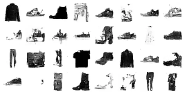

Stable Diffusion (Text-to-Image)

Cuối cùng, chúng ta sẽ trải nghiệm sức mạnh của một mô hình Diffusion tiên tiến nhất hiện nay: Stable Diffusion. Đây là mô hình Latent Diffusion, hoạt động trên không gian latent thay vì pixel để tiết kiệm tài nguyên.

Chúng ta sử dụng thư viện diffusers của Hugging Face.

from diffusers import AutoPipelineForText2Image

# Tải mô hình SD-Turbo (phiên bản siêu nhanh)
pipe = AutoPipelineForText2Image.from_pretrained(
    "stabilityai/sd-turbo", variant="fp16", dtype=torch.float16)
pipe.to(device)
prompt = "A closeup photo of an orangutan reading a book"

output:
    ...
    Loading pipeline components...:   0%|          | 0/5 [00:00<?, ?it/s]

torch.manual_seed(42)
# Sinh ảnh từ văn bản chỉ trong 1 bước suy luận
image = pipe(prompt=prompt, num_inference_steps=1, guidance_scale=0.0).images[0]
image.save("my_orangutan_reading.png")
plt.imshow(image)
plt.axis("off")
plt.show()

output:
    0%|          | 0/1 [00:00<?, ?it/s]