[ML101] Chương 8: Học Không Giám Sát (Unsupervised Learning)
K-Means, DBSCAN và các thuật toán clustering
Bài viết có tham khảo, sử dụng và sửa đổi tài nguyên từ kho lưu trữ handson-mlp, tuân thủ giấy phép Apache‑2.0. Chúng tôi chân thành cảm ơn tác giả Aurélien Géron (@aureliengeron) vì sự chia sẻ kiến thức tuyệt vời và những đóng góp quý giá cho cộng đồng.
Trong các chương trước, chúng ta chủ yếu tập trung vào Học có giám sát (Supervised Learning), nơi mục tiêu là dự đoán nhãn (label) từ dữ liệu đầu vào. Tuy nhiên, trong thực tế, dữ liệu được gán nhãn thường rất ít và tốn kém để tạo ra, trong khi dữ liệu chưa gán nhãn lại vô cùng phong phú. Học không giám sát (Unsupervised Learning) giải quyết vấn đề này bằng cách tìm ra các mẫu (patterns), cấu trúc hoặc tri thức ẩn giấu bên trong dữ liệu mà không cần bất kỳ nhãn nào.
Chương này sẽ đi sâu vào các kỹ thuật quan trọng nhất của học không giám sát, bao gồm:
- Phân cụm (Clustering): Gom nhóm các dữ liệu tương đồng nhau.
- Phát hiện bất thường (Anomaly Detection): Tìm kiếm các điểm dữ liệu khác biệt so với phần còn lại.
- Ước lượng mật độ (Density Estimation): Ước tính hàm phân phối xác suất của dữ liệu.
Bạn có thể chạy trực tiếp các đoạn mã code tại: Google Colab.
Cài đặt môi trường
Trước tiên, vẫn như thường lệ, chúng ta cần đảm bảo môi trường Python và các thư viện cần thiết như Scikit-Learn và Matplotlib được cài đặt đúng phiên bản để đảm bảo mã nguồn chạy ổn định.
# Yêu cầu Python 3.10 trở lên
import sys
assert sys.version_info >= (3, 10)

# Yêu cầu Scikit-Learn phiên bản 1.6.1 trở lên
from packaging.version import Version
import sklearn
assert Version(sklearn.__version__) >= Version("1.6.1")

# Thiết lập kích thước font chữ mặc định cho biểu đồ Matplotlib để dễ nhìn hơn
import matplotlib.pyplot as plt

plt.rc('font', size=14)
plt.rc('axes', labelsize=14, titlesize=14)
plt.rc('legend', fontsize=14)
plt.rc('xtick', labelsize=10)
plt.rc('ytick', labelsize=10)
1. Phân cụm (Clustering)
Giới thiệu – Phân loại (Classification) so với Phân cụm (Clustering)
Để hiểu rõ sự khác biệt, hãy xem xét bộ dữ liệu hoa Iris.
- Bên trái (Phân loại): Mỗi điểm dữ liệu đi kèm với một nhãn cụ thể (loài hoa). Các thuật toán như Logistic Regression hay SVM sẽ tìm đường ranh giới (decision boundary) để phân chia các lớp này.
- Bên phải (Phân cụm): Chúng ta không có nhãn. Dữ liệu chỉ là các điểm trong không gian. Nhiệm vụ của thuật toán phân cụm là tự động phát hiện ra các nhóm dữ liệu tụ tập lại với nhau dựa trên độ tương đồng (similarity) hoặc khoảng cách.
# extra code – đoạn này tạo Hình 8–1
import matplotlib.pyplot as plt
from sklearn.datasets import load_iris

# Tải dữ liệu Iris
data = load_iris()
X = data.data
y = data.target
data.target_names

plt.figure(figsize=(9, 3.5))

# Biểu đồ bên trái: Dữ liệu có nhãn (Classification)
plt.subplot(121)
plt.plot(X[y==0, 2], X[y==0, 3], "yo", label="Iris setosa")
plt.plot(X[y==1, 2], X[y==1, 3], "bs", label="Iris versicolor")
plt.plot(X[y==2, 2], X[y==2, 3], "g^", label="Iris virginica")
plt.xlabel("Petal length")
plt.ylabel("Petal width")
plt.grid()
plt.legend()

# Biểu đồ bên phải: Dữ liệu không nhãn (Clustering)
plt.subplot(122)
plt.scatter(X[:, 2], X[:, 3], c="k", marker=".")
plt.xlabel("Petal length")
plt.tick_params(labelleft=False)
plt.gca().set_axisbelow(True)
plt.grid()

plt.show()
Dưới đây là một ví dụ minh họa trước về việc sử dụng Mô hình Hỗn hợp Gaussian (Gaussian Mixture Model - GMM) để phân tách các cụm này. GMM giả định dữ liệu được sinh ra từ hỗn hợp của nhiều phân phối Gaussian (hình chuông).
Đoạn mã sau sử dụng GMM để gom nhóm, sau đó ánh xạ (map) mỗi cụm tìm được với loài hoa phổ biến nhất trong cụm đó để so sánh với nhãn thực tế.
# extra code
import numpy as np
from scipy import stats
from sklearn.mixture import GaussianMixture

# Sử dụng GMM để phân cụm
y_pred = GaussianMixture(n_components=3, random_state=42).fit(X).predict(X)

# Ánh xạ từng cụm sang lớp (loài hoa) phổ biến nhất trong cụm đó
mapping = {}
for class_id in np.unique(y):
    mode, _ = stats.mode(y_pred[y==class_id])
    mapping[mode] = class_id

y_pred = np.array([mapping[cluster_id] for cluster_id in y_pred])

# Vẽ kết quả phân cụm
plt.plot(X[y_pred==0, 2], X[y_pred==0, 3], "yo", label="Cluster 1")
plt.plot(X[y_pred==1, 2], X[y_pred==1, 3], "bs", label="Cluster 2")
plt.plot(X[y_pred==2, 2], X[y_pred==2, 3], "g^", label="Cluster 3")
plt.xlabel("Petal length")
plt.ylabel("Petal width")
plt.legend(loc="upper left")
plt.grid()
plt.show()
Chúng ta có thể kiểm tra tỷ lệ các mẫu hoa Iris được gán đúng cụm (tương ứng với nhãn thực tế). Kết quả cho thấy độ chính xác rất cao, lên tới khoảng 96.6%.
# Tính tỷ lệ phần trăm mẫu được gán đúng cụm
(y_pred==y).sum() / len(y_pred)
output:
np.float64(0.9666666666666667)K-Means (K-Trung bình)
K-Means là một thuật toán đơn giản và hiệu quả, có khả năng phân cụm dữ liệu rất nhanh. Ý tưởng chính là tìm ra tâm cụm (centroids) và gán mỗi điểm dữ liệu vào tâm cụm gần nhất. Mục tiêu toán học là tối thiểu hóa tổng bình phương khoảng cách (inertia) trong mỗi cụm:
Huấn luyện và Dự đoán
Hãy bắt đầu bằng việc tạo ra một bộ dữ liệu giả lập gồm 5 nhóm (blobs) và huấn luyện mô hình K-Means.
from sklearn.cluster import KMeans
from sklearn.datasets import make_blobs

# extra code – tạo dữ liệu blobs giả lập
blob_centers = np.array([[ 0.2,  2.3], [-1.5 ,  2.3], [-2.8,  1.8],
                         [-2.8,  2.8], [-2.8,  1.3]])
blob_std = np.array([0.4, 0.3, 0.1, 0.1, 0.1])
X, y = make_blobs(n_samples=2000, centers=blob_centers, cluster_std=blob_std,
                  random_state=7)

# Huấn luyện K-Means với k=5
k = 5
kmeans = KMeans(n_clusters=k, random_state=43)
y_pred = kmeans.fit_predict(X)
Sau khi huấn luyện, chúng ta có thể trực quan hóa các cụm mà K-Means đã tìm thấy. Lưu ý rằng thuật toán không biết nhãn thực sự, nó chỉ gom nhóm dựa trên khoảng cách.
# extra code – hàm vẽ biểu đồ các cụm
def plot_clusters(X, y=None):
    plt.scatter(X[:, 0], X[:, 1], c=y, s=1)
    plt.xlabel("$x_1$")
    plt.ylabel("$x_2$", rotation=0)

plt.figure(figsize=(8, 4))
plot_clusters(X)
plt.gca().set_axisbelow(True)
plt.grid()
plt.show()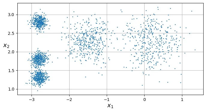
Mỗi điểm dữ liệu đã được gán một nhãn (từ 0 đến 4), đại diện cho chỉ số của cụm mà nó thuộc về. Bạn có thể truy cập các nhãn này thông qua thuộc tính labels_.
y_predoutput:
array([4, 0, 1, ..., 2, 1, 0], dtype=int32)y_pred is kmeans.labels_output:
TrueChúng ta cũng có thể xem tọa độ của 5 tâm cụm (centroids) mà thuật toán đã ước lượng được:
kmeans.cluster_centers_output:
array([[-2.80389616, 1.80117999],
[ 0.20876306, 2.25551336],
[-2.79290307, 2.79641063],
[-1.46679593, 2.28585348],
[-2.80037642, 1.30082566]])Một điều cần lưu ý: nhãn cụm (0, 1, 2…) là ngẫu nhiên và phụ thuộc vào thứ tự khởi tạo, chúng không mang ý nghĩa ngữ nghĩa như “nhãn lớp” trong học có giám sát.
kmeans.labels_output:
array([4, 0, 1, ..., 2, 1, 0], dtype=int32)Tất nhiên, bạn có thể sử dụng mô hình đã huấn luyện để dự đoán cụm cho các điểm dữ liệu mới:
import numpy as np
X_new = np.array([[0, 2], [3, 2], [-3, 3], [-3, 2.5]])
kmeans.predict(X_new)
output:
array([1, 1, 2, 2], dtype=int32)Ranh giới Quyết định (Decision Boundaries)
Khi vẽ ranh giới quyết định của K-Means, chúng ta sẽ nhận được một biểu đồ Voronoi (Voronoi diagram). Không gian được chia thành các ô, trong đó mọi điểm trong một ô đều gần tâm cụm của ô đó hơn bất kỳ tâm cụm nào khác.
# extra code – hàm vẽ ranh giới quyết định và tâm cụm
def plot_data(X):
    plt.plot(X[:, 0], X[:, 1], 'k.', markersize=2)

def plot_centroids(centroids, weights=None, circle_color='w', cross_color='k'):
    if weights is not None:
        centroids = centroids[weights > weights.max() / 10]
    plt.scatter(centroids[:, 0], centroids[:, 1],
                marker='o', s=35, linewidths=8,
                color=circle_color, zorder=10, alpha=0.9)
    plt.scatter(centroids[:, 0], centroids[:, 1],
                marker='x', s=2, linewidths=12,
                color=cross_color, zorder=11, alpha=1)

def plot_decision_boundaries(clusterer, X, resolution=1000, show_centroids=True,
                             show_xlabels=True, show_ylabels=True):
    mins = X.min(axis=0) - 0.1
    maxs = X.max(axis=0) + 0.1
    xx, yy = np.meshgrid(np.linspace(mins[0], maxs[0], resolution),
                         np.linspace(mins[1], maxs[1], resolution))
    Z = clusterer.predict(np.c_[xx.ravel(), yy.ravel()])
    Z = Z.reshape(xx.shape)

    plt.contourf(Z, extent=(mins[0], maxs[0], mins[1], maxs[1]),
                cmap="Pastel2")
    plt.contour(Z, extent=(mins[0], maxs[0], mins[1], maxs[1]),
                linewidths=1, colors='k')
    plot_data(X)
    if show_centroids:
        plot_centroids(clusterer.cluster_centers_)

    if show_xlabels:
        plt.xlabel("$x_1$")
    else:
        plt.tick_params(labelbottom=False)
    if show_ylabels:
        plt.ylabel("$x_2$", rotation=0)
    else:
        plt.tick_params(labelleft=False)

plt.figure(figsize=(8, 4))
plot_decision_boundaries(kmeans, X)
plt.show()
Phân cụm Cứng (Hard Clustering) so với Phân cụm Mềm (Soft Clustering)
- Phân cụm cứng: Gán mỗi điểm dữ liệu vào duy nhất một cụm.
- Phân cụm mềm: Tính toán điểm số (thường là khoảng cách hoặc độ tương đồng) của mỗi điểm dữ liệu đối với tất cả các cụm.
Phương thức transform() trong Scikit-Learn trả về khoảng cách Euclidean từ điểm dữ liệu đến từng tâm cụm.
# Tính khoảng cách từ các điểm mới đến 5 tâm cụm
kmeans.transform(X_new).round(2)
output:
array([[2.81, 0.33, 2.9 , 1.49, 2.89],
[5.81, 2.8 , 5.85, 4.48, 5.84],
[1.21, 3.29, 0.29, 1.69, 1.71],
[0.73, 3.22, 0.36, 1.55, 1.22]])Bạn có thể xác minh rằng kết quả trên chính xác là khoảng cách Euclidean:
# extra code - Kiểm tra thủ công khoảng cách Euclidean
np.linalg.norm(np.tile(X_new, (1, k)).reshape(-1, k, 2)
               - kmeans.cluster_centers_, axis=2).round(2)
output:
array([[2.81, 0.33, 2.9 , 1.49, 2.89],
[5.81, 2.8 , 5.85, 4.48, 5.84],
[1.21, 3.29, 0.29, 1.69, 1.71],
[0.73, 3.22, 0.36, 1.55, 1.22]])Thuật toán K-Means
Thuật toán K-Means hoạt động theo quy trình lặp đi lặp lại rất đơn giản (Expectation-Maximization):
- Khởi tạo: Chọn ngẫu nhiên điểm làm tâm cụm ban đầu (centroids).
- Lặp cho đến khi hội tụ (tâm cụm không thay đổi nữa):
- Gán (Expectation step): Gán mỗi điểm dữ liệu vào tâm cụm gần nhất.
- Cập nhật (Maximization step): Tính lại vị trí tâm cụm bằng trung bình cộng (mean) của tất cả các điểm thuộc cụm đó.
Dưới đây, chúng ta sẽ mô phỏng quá trình này qua 3 vòng lặp đầu tiên để xem các tâm cụm di chuyển như thế nào.
# extra code – tạo hình 8–4 mô phỏng các bước lặp của K-Means
kmeans_iter1 = KMeans(n_clusters=5, init="random", n_init=1, max_iter=1,
                      random_state=18)
kmeans_iter2 = KMeans(n_clusters=5, init="random", n_init=1, max_iter=2,
                      random_state=18)
kmeans_iter3 = KMeans(n_clusters=5, init="random", n_init=1, max_iter=3,
                      random_state=18)
kmeans_iter1.fit(X)
kmeans_iter2.fit(X)
kmeans_iter3.fit(X)

plt.figure(figsize=(10, 8))

plt.subplot(321)
plot_data(X)
plot_centroids(kmeans_iter1.cluster_centers_, circle_color='r', cross_color='w')
plt.ylabel("$x_2$", rotation=0)
plt.tick_params(labelbottom=False)
plt.title("Update the centroids (initially randomly)")

plt.subplot(322)
plot_decision_boundaries(kmeans_iter1, X, show_xlabels=False,
                         show_ylabels=False)
plt.title("Label the instances")

plt.subplot(323)
plot_decision_boundaries(kmeans_iter1, X, show_centroids=False,
                         show_xlabels=False)
plot_centroids(kmeans_iter2.cluster_centers_)

plt.subplot(324)
plot_decision_boundaries(kmeans_iter2, X, show_xlabels=False,
                         show_ylabels=False)

plt.subplot(325)
plot_decision_boundaries(kmeans_iter2, X, show_centroids=False)
plot_centroids(kmeans_iter3.cluster_centers_)

plt.subplot(326)
plot_decision_boundaries(kmeans_iter3, X, show_ylabels=False)

plt.show()
Sự biến thiên của K-Means (K-Means Variability)
Vấn đề lớn nhất của K-Means cơ bản là sự phụ thuộc vào khởi tạo ngẫu nhiên. Nếu xui xẻo chọn phải các tâm cụm ban đầu không tốt, thuật toán có thể hội tụ tại một cực trị địa phương (local optimum) thay vì giải pháp tốt nhất toàn cục (global optimum).
Dưới đây là ví dụ về hai lần chạy với khởi tạo ngẫu nhiên khác nhau dẫn đến hai kết quả phân cụm khác hẳn nhau (và đều không tối ưu).
# extra code – tạo hình 8–5 so sánh các khởi tạo khác nhau
def plot_clusterer_comparison(clusterer1, clusterer2, X, title1=None,
                              title2=None):
    clusterer1.fit(X)
    clusterer2.fit(X)

    plt.figure(figsize=(10, 3.2))

    plt.subplot(121)
    plot_decision_boundaries(clusterer1, X)
    if title1:
        plt.title(title1)

    plt.subplot(122)
    plot_decision_boundaries(clusterer2, X, show_ylabels=False)
    if title2:
        plt.title(title2)

kmeans_rnd_init1 = KMeans(n_clusters=5, init="random", n_init=1, random_state=2)
kmeans_rnd_init2 = KMeans(n_clusters=5, init="random", n_init=1, random_state=8)

plot_clusterer_comparison(kmeans_rnd_init1, kmeans_rnd_init2, X,
                          "Solution 1",
                          "Solution 2 (with a different random init)")

plt.show()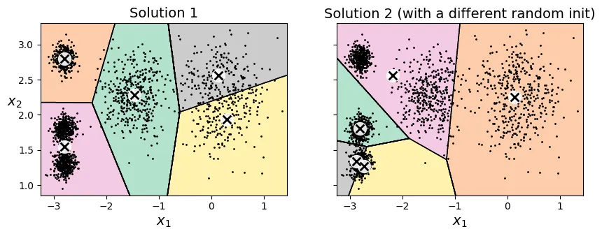
Nếu bạn biết trước vị trí gần đúng của các tâm cụm, bạn có thể truyền chúng vào tham số init để hướng dẫn thuật toán, giúp nó hội tụ đúng chỗ.
# Khởi tạo thủ công các tâm cụm
good_init = np.array([[-3, 3], [-3, 2], [-3, 1], [-1, 2], [0, 2]])
kmeans = KMeans(n_clusters=5, init=good_init, random_state=42)
kmeans.fit(X)
output:
KMeans(init=array([[-3, 3],
[-3, 2],
[-3, 1],
[-1, 2],
[ 0, 2]]),
n_clusters=5, random_state=42)# extra code - vẽ kết quả khởi tạo tốt
plt.figure(figsize=(8, 4))
plot_decision_boundaries(kmeans, X)
Quán tính (Inertia)
Để đánh giá xem mô hình K-Means tốt hay xấu (vì không có nhãn để so sánh), chúng ta sử dụng một chỉ số gọi là Quán tính (Inertia).
Inertia chính là tổng bình phương khoảng cách giữa mỗi điểm dữ liệu và tâm cụm gần nhất của nó. Inertia càng nhỏ, các điểm càng nằm gần tâm cụm, nghĩa là cụm càng chặt chẽ.
kmeans.inertia_output:
211.59853725816828Hãy so sánh Inertia của mô hình tốt với hai mô hình khởi tạo ngẫu nhiên xấu ở trên. Bạn sẽ thấy Inertia của mô hình tốt thấp hơn nhiều.
kmeans_rnd_init1.inertia_ # extra codeoutput:
219.58201503602285kmeans_rnd_init2.inertia_ # extra codeoutput:
600.3600713094229Lưu ý rằng phương thức score() trong Scikit-Learn trả về giá trị Inertia âm. Lý do là vì quy tắc chung của thư viện này là “điểm càng cao càng tốt” (như accuracy), trong khi Inertia thì “càng thấp càng tốt”.
kmeans.score(X)output:
-211.59853725816828Đa khởi tạo (Multiple Initializations)
Để giải quyết vấn đề hội tụ sai, giải pháp đơn giản nhất là chạy thuật toán nhiều lần với các khởi tạo ngẫu nhiên khác nhau và chọn mô hình có Inertia thấp nhất.
Trong Scikit-Learn, tham số n_init kiểm soát số lần chạy này. Theo mặc định, KMeans sẽ chạy thuật toán nhiều lần và giữ lại kết quả tốt nhất.
# extra code
kmeans_rnd_10_inits = KMeans(n_clusters=5, init="random", n_init=10,
                             random_state=2)
kmeans_rnd_10_inits.fit(X)
output:
KMeans(init='random', n_clusters=5, n_init=10, random_state=2)# extra code - vẽ kết quả sau khi chạy 10 lần khởi tạo
plt.figure(figsize=(8, 4))
plot_decision_boundaries(kmeans_rnd_10_inits, X)
plt.show()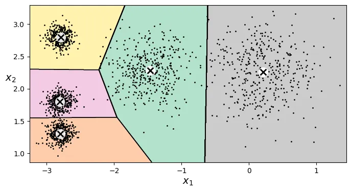
Phương pháp khởi tạo K-Means++
Thay vì chọn ngẫu nhiên hoàn toàn, thuật toán K-Means++ chọn các tâm cụm ban đầu sao cho chúng nằm xa nhau nhất có thể. Điều này giúp thuật toán hội tụ nhanh hơn và tránh được các giải pháp tối ưu cục bộ tồi tệ.
Scikit-Learn sử dụng init="k-means++" làm mặc định. Nếu muốn dùng khởi tạo ngẫu nhiên thuần túy, bạn phải set init="random".
K-Means Tăng tốc (Accelerated K-Means) và Mini-Batch K-Means
Có những biến thể của K-Means giúp chạy nhanh hơn:
- Accelerated K-Means (Elkan’s algorithm): Tránh các phép tính khoảng cách không cần thiết bằng cách sử dụng bất đẳng thức tam giác. Đây là mặc định trong Scikit-Learn (
algorithm="elkan"hoặc"lloyd"). - Mini-Batch K-Means: Thay vì dùng toàn bộ dữ liệu ở mỗi bước lặp, nó chỉ dùng các lô nhỏ (mini-batches). Điều này giúp thuật toán chạy nhanh hơn nhiều trên dữ liệu lớn, dù Inertia có thể cao hơn một chút.
from sklearn.cluster import MiniBatchKMeans

# Sử dụng Mini-Batch K-Means
minibatch_kmeans = MiniBatchKMeans(n_clusters=5, random_state=42)
minibatch_kmeans.fit(X)
output:
MiniBatchKMeans(n_clusters=5, random_state=42)minibatch_kmeans.inertia_output:
211.65945105712612Sử dụng MiniBatchKMeans với memmap
Khi dữ liệu quá lớn không thể nạp hết vào RAM, chúng ta có thể dùng np.memmap (memory mapping) để ánh xạ file trên đĩa cứng vào bộ nhớ, cho phép MiniBatchKMeans xử lý dữ liệu từng phần.
from sklearn.datasets import fetch_openml

# Tải dữ liệu MNIST
mnist = fetch_openml('mnist_784', as_frame=False)

# Chia tập train/test
X_train, y_train = mnist.data[:60000], mnist.target[:60000]
X_test, y_test = mnist.data[60000:], mnist.target[60000:]

# Tạo file memmap
filename = "my_mnist.mmap"
X_memmap = np.memmap(filename, dtype='float32', mode='write',
                     shape=X_train.shape)
X_memmap[:] = X_train
X_memmap.flush()

# Huấn luyện MiniBatchKMeans trên dữ liệu memmap
minibatch_kmeans = MiniBatchKMeans(n_clusters=10, batch_size=10,
                                   random_state=42)
minibatch_kmeans.fit(X_memmap)
output:
MiniBatchKMeans(batch_size=10, n_clusters=10, random_state=42)Tìm số lượng cụm tối ưu ()
Việc chọn là một bài toán khó. Nếu chọn quá nhỏ hoặc quá lớn, kết quả phân cụm sẽ không tốt. Dưới đây là ví dụ khi chọn và cho dữ liệu 5 cụm.
# extra code – tạo hình 8–6 so sánh k=3 và k=8
kmeans_k3 = KMeans(n_clusters=3, random_state=42)
kmeans_k8 = KMeans(n_clusters=8, random_state=42)

plot_clusterer_comparison(kmeans_k3, kmeans_k8, X, "$k=3$", "$k=8$")
plt.show()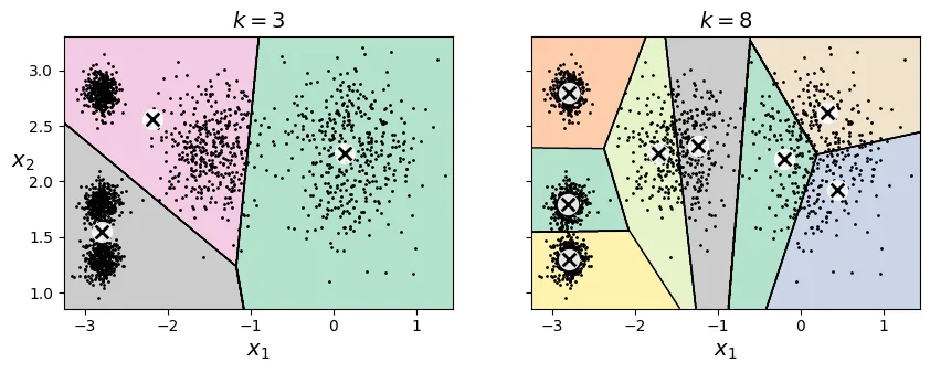
Chúng ta không thể chỉ dựa vào việc giảm thiểu Inertia để chọn , vì Inertia sẽ luôn giảm khi tăng (càng nhiều cụm, các điểm càng gần tâm cụm của nó).
Một phương pháp phổ biến là Quy tắc Khuỷu tay (Elbow Rule): Vẽ biểu đồ Inertia theo và tìm điểm gập khúc (như khuỷu tay), nơi mà việc tăng không còn làm giảm Inertia đáng kể nữa.
# extra code – tạo hình 8–8 biểu đồ Inertia
kmeans_per_k = [KMeans(n_clusters=k, random_state=43).fit(X)
                for k in range(1, 10)]
inertias = [model.inertia_ for model in kmeans_per_k]

plt.figure(figsize=(8, 3.5))
plt.plot(range(1, 10), inertias, "bo-")
plt.xlabel("$k$")
plt.ylabel("Inertia")
plt.annotate("", xy=(4, inertias[3]), xytext=(4.45, 650),
             arrowprops=dict(facecolor='black', shrink=0.1))
plt.text(4.5, 650, "Elbow", horizontalalignment="center")
plt.axis([1, 8.5, 0, 1300])
plt.grid()
plt.show()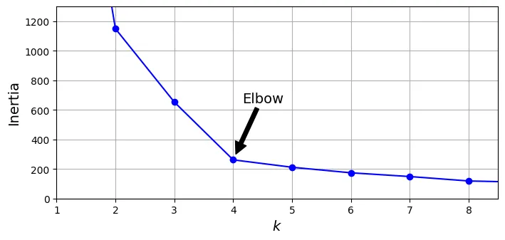
Tại , ta thấy một “khuỷu tay”. Điều này cho thấy hoặc là lựa chọn hợp lý.
Điểm số Dáng điệu (Silhouette Score)
Một phương pháp chính xác hơn là sử dụng Hệ số Dáng điệu (Silhouette Coefficient). Hệ số này đo lường mức độ giống nhau của một điểm với cụm của nó so với các cụm khác. Trong đó:
-
: Khoảng cách trung bình giữa điểm đó và các điểm khác trong cùng cụm.
-
: Khoảng cách trung bình giữa điểm đó và các điểm trong cụm gần nhất.
-
Giá trị gần +1: Điểm nằm gọn trong cụm của nó và xa các cụm khác (tốt).
-
Giá trị gần 0: Điểm nằm ở biên giới giữa các cụm.
-
Giá trị gần -1: Điểm có thể đã bị gán nhầm cụm.
Silhouette Score là trung bình của hệ số này trên toàn bộ dữ liệu.
from sklearn.metrics import silhouette_score
silhouette_score(X, kmeans.labels_)
output:
0.655517642572828Hãy vẽ biểu đồ Silhouette Score theo . Giá trị cao nhất sẽ là tốt nhất.
# extra code – tạo hình 8–9
silhouette_scores = [silhouette_score(X, model.labels_)
                     for model in kmeans_per_k[1:]]

plt.figure(figsize=(8, 3))
plt.plot(range(2, 10), silhouette_scores, "bo-")
plt.xlabel("$k$")
plt.ylabel("Silhouette score")
plt.axis([1.8, 8.5, 0.55, 0.7])
plt.grid()
plt.show()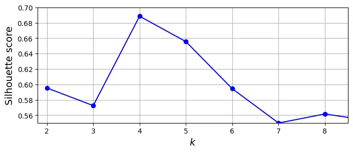
Biểu đồ cho thấy và đều rất tốt. Để phân tích sâu hơn, ta dùng Biểu đồ Dáng điệu (Silhouette Diagram).
Trong biểu đồ này, mỗi cụm được biểu diễn bằng hình dạng con dao. Chiều rộng biểu thị số lượng mẫu, chiều dài biểu thị hệ số silhouette. Đường nét đứt màu đỏ là điểm số trung bình.
- Nếu hầu hết các mẫu trong cụm đều vượt qua đường đỏ: Cụm tốt.
- Nếu các cụm có kích thước đồng đều: Phân cụm cân bằng.
# extra code – tạo hình 8–10 (Silhouette Diagram)
from sklearn.metrics import silhouette_samples
from matplotlib.ticker import FixedLocator, FixedFormatter

plt.figure(figsize=(11, 9))

for k in (3, 4, 5, 6):
    plt.subplot(2, 2, k - 2)

    y_pred = kmeans_per_k[k - 1].labels_
    silhouette_coefficients = silhouette_samples(X, y_pred)

    padding = len(X) // 30
    pos = padding
    ticks = []
    for i in range(k):
        coeffs = silhouette_coefficients[y_pred == i]
        coeffs.sort()

        color = plt.cm.Spectral(i / k)
        plt.fill_betweenx(np.arange(pos, pos + len(coeffs)), 0, coeffs,
                          facecolor=color, edgecolor=color, alpha=0.7)
        ticks.append(pos + len(coeffs) // 2)
        pos += len(coeffs) + padding

    plt.gca().yaxis.set_major_locator(FixedLocator(ticks))
    plt.gca().yaxis.set_major_formatter(FixedFormatter(range(k)))
    if k in (3, 5):
        plt.ylabel("Cluster")

    if k in (5, 6):
        plt.gca().set_xticks([-0.1, 0, 0.2, 0.4, 0.6, 0.8, 1])
        plt.xlabel("Silhouette Coefficient")
    else:
        plt.tick_params(labelbottom=False)

    plt.axvline(x=silhouette_scores[k - 2], color="red", linestyle="--")
    plt.title(f"$k={k}$")

plt.show()
Nhìn vào biểu đồ, tại , các cụm có kích thước tương đối đều nhau và hầu hết các điểm đều vượt qua ngưỡng trung bình. Đây là lựa chọn tốt nhất.
Hạn chế của K-Means
K-Means hoạt động tốt nhất trên các cụm hình cầu, có kích thước và mật độ tương đương nhau. Khi các cụm có hình dạng méo mó (elongated), mật độ khác nhau, hoặc kích thước chênh lệch, K-Means thường thất bại do nó dựa trên khoảng cách Euclidean.
# extra code – tạo hình 8–11 minh họa hạn chế của K-Means
X1, y1 = make_blobs(n_samples=1000, centers=((4, -4), (0, 0)), random_state=42)
X1 = X1.dot(np.array([[0.374, 0.95], [0.732, 0.598]]))
X2, y2 = make_blobs(n_samples=250, centers=1, random_state=42)
X2 = X2 + [6, -8]
X = np.r_[X1, X2]
y = np.r_[y1, y2]

kmeans_good = KMeans(n_clusters=3,
                     init=np.array([[-1.5, 2.5], [0.5, 0], [4, 0]]),
                     random_state=42)
kmeans_bad = KMeans(n_clusters=3, n_init=10, random_state=42)
kmeans_good.fit(X)
kmeans_bad.fit(X)

plt.figure(figsize=(10, 3.2))

plt.subplot(121)
plot_decision_boundaries(kmeans_good, X)
plt.title(f"Inertia = {kmeans_good.inertia_:.1f}")

plt.subplot(122)
plot_decision_boundaries(kmeans_bad, X, show_ylabels=False)
plt.title(f"Inertia = {kmeans_bad.inertia_:.1f}")

plt.show()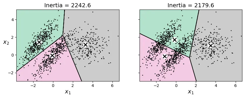
2. Ứng dụng: Phân đoạn Ảnh (Image Segmentation)
Một ứng dụng thú vị của K-Means là phân đoạn ảnh, cụ thể là lượng tử hóa màu (color quantization). Chúng ta sẽ giảm số lượng màu trong ảnh xuống còn màu, bằng cách gôm nhóm các pixel có màu sắc tương tự nhau.
# extra code – tải ảnh con bọ rùa (ladybug)
from pathlib import Path
import urllib.request

homlp_root = "https://github.com/ageron/handson-mlp/raw/main/"
filename = "ladybug.png"
filepath = Path(f"my_{filename}")
if not filepath.is_file():
    print("Downloading", filename)
    url = f"{homlp_root}/images/unsupervised_learning/{filename}"
    urllib.request.urlretrieve(url, filepath)
import PIL
image = np.asarray(PIL.Image.open(filepath))
image.shapeoutput:
(533, 800, 3)Mỗi pixel là một điểm dữ liệu 3 chiều (Red, Green, Blue). Chúng ta sẽ dùng K-Means để tìm ra 8 màu chủ đạo và thay thế toàn bộ pixel trong ảnh bằng màu của tâm cụm gần nhất.
X = image.reshape(-1, 3)
kmeans = KMeans(n_clusters=8, random_state=42).fit(X)
segmented_img = kmeans.cluster_centers_[kmeans.labels_]
segmented_img = segmented_img.reshape(image.shape)
# extra code – tạo hình 8–12 so sánh số lượng màu khác nhau
segmented_imgs = []
n_colors = (10, 8, 6, 4, 2)
for n_clusters in n_colors:
kmeans = KMeans(n_clusters=n_clusters, random_state=42).fit(X)
segmented_img = kmeans.cluster_centers_[kmeans.labels_]
segmented_imgs.append(segmented_img.reshape(image.shape))
plt.figure(figsize=(10, 5))
plt.subplots_adjust(wspace=0.05, hspace=0.1)
plt.subplot(2, 3, 1)
plt.imshow(image)
plt.title("Original image")
plt.axis('off')
for idx, n_clusters in enumerate(n_colors):
plt.subplot(2, 3, 2 + idx)
plt.imshow(segmented_imgs[idx] / 255)
plt.title(f"{n_clusters} colors")
plt.axis('off')
plt.show()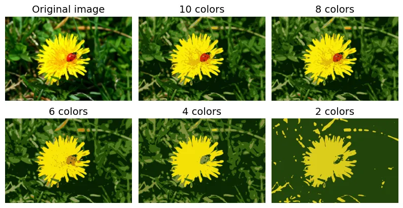
3. Ứng dụng: Học Bán Giám Sát (Semi-Supervised Learning)
Giả sử chúng ta có bộ dữ liệu số viết tay (Digits), nhưng chỉ có rất ít nhãn. Làm thế nào để đạt độ chính xác cao? Đây là bài toán Semi-Supervised Learning.
Đầu tiên, tải dữ liệu và chia tập train/test:
from sklearn.datasets import load_digits

X_digits, y_digits = load_digits(return_X_y=True)
X_train, y_train = X_digits[:1400], y_digits[:1400]
X_test, y_test = X_digits[1400:], y_digits[1400:]
Nếu chỉ huấn luyện mô hình (ví dụ: Logistic Regression) trên 50 mẫu dữ liệu được gán nhãn ngẫu nhiên, độ chính xác sẽ khá thấp.
from sklearn.linear_model import LogisticRegression

n_labeled = 50
log_reg = LogisticRegression(max_iter=10_000)
log_reg.fit(X_train[:n_labeled], y_train[:n_labeled])
output:
LogisticRegression(max_iter=10000)log_reg.score(X_test, y_test)output:
0.7581863979848866So với việc huấn luyện trên toàn bộ dữ liệu (để tham chiếu):
# extra code – độ chính xác khi dùng toàn bộ dữ liệu
log_reg_full = LogisticRegression(max_iter=10_000)
log_reg_full.fit(X_train, y_train)
log_reg_full.score(X_test, y_test)
output:
0.9093198992443325Cải thiện bằng cách chọn mẫu đại diện
Thay vì chọn 50 mẫu ngẫu nhiên, chúng ta sẽ phân cụm dữ liệu thành 50 cụm, sau đó tìm ảnh đại diện (representative image) của mỗi cụm (ảnh gần tâm cụm nhất). Việc gán nhãn cho 50 ảnh đại diện này sẽ mang lại nhiều thông tin hơn là 50 ảnh ngẫu nhiên.
k = 50
kmeans = KMeans(n_clusters=k, random_state=42)
X_digits_dist = kmeans.fit_transform(X_train)
representative_digit_idx = X_digits_dist.argmin(axis=0)
X_representative_digits = X_train[representative_digit_idx]
# extra code – hiển thị 50 ảnh đại diện của các cụm
plt.figure(figsize=(8, 2))
for index, X_representative_digit in enumerate(X_representative_digits):
plt.subplot(k // 10, 10, index + 1)
plt.imshow(X_representative_digit.reshape(8, 8), cmap="binary",
interpolation="bilinear")
plt.axis('off')
plt.show()
Tiếp theo, ta giả lập việc gán nhãn thủ công cho 50 ảnh này:
y_representative_digits = np.array([
    8, 0, 1, 3, 6, 7, 5, 4, 2, 8,
    2, 3, 9, 5, 3, 9, 1, 7, 9, 1,
    4, 6, 9, 7, 5, 2, 2, 1, 3, 3,
    6, 0, 4, 9, 8, 1, 8, 4, 2, 4,
    2, 3, 9, 7, 8, 9, 6, 5, 6, 4,])
Bây giờ hãy huấn luyện lại mô hình với 50 mẫu đại diện này:
log_reg = LogisticRegression(max_iter=10_000)
log_reg.fit(X_representative_digits, y_representative_digits)
log_reg.score(X_test, y_test)
output:
0.8337531486146096Độ chính xác tăng vọt! Từ khoảng 75.8% lên 83.4%. Điều này cho thấy chọn mẫu thông minh (dựa trên phân cụm) tốt hơn chọn ngẫu nhiên.
Lan truyền nhãn (Label Propagation)
Chúng ta có thể làm tốt hơn nữa bằng cách lan truyền nhãn của mẫu đại diện cho tất cả các mẫu khác trong cùng cụm đó.
y_train_propagated = np.empty(len(X_train), dtype=np.int64)
for i in range(k):
    y_train_propagated[kmeans.labels_ == i] = y_representative_digits[i]

log_reg = LogisticRegression(max_iter=10_000)
log_reg.fit(X_train, y_train_propagated)
log_reg.score(X_test, y_test)
output:
0.8690176322418136Kết quả tiếp tục tăng! Tuy nhiên, việc lan truyền nhãn cho các điểm ở rìa cụm (xa tâm) có thể gây nhiễu vì chúng dễ bị phân loại sai. Hãy thử chỉ lan truyền cho 50% các điểm gần tâm nhất.
percentile_closest = 50
X_cluster_dist = X_digits_dist[np.arange(len(X_train)), kmeans.labels_]
for i in range(k):
    in_cluster = (kmeans.labels_ == i)
    cluster_dist = X_cluster_dist[in_cluster]
    cutoff_distance = np.percentile(cluster_dist, percentile_closest)
    above_cutoff = (X_cluster_dist > cutoff_distance)
    X_cluster_dist[in_cluster & above_cutoff] = -1

partially_propagated = (X_cluster_dist != -1)
X_train_partially_propagated = X_train[partially_propagated]
y_train_partially_propagated = y_train_propagated[partially_propagated]

log_reg = LogisticRegression(max_iter=10_000)
log_reg.fit(X_train_partially_propagated, y_train_partially_propagated)
log_reg.score(X_test, y_test)
output:
0.8841309823677582Độ chính xác đạt mức rất ấn tượng (~88.4%) chỉ với 50 nhãn gốc ban đầu!
(y_train_partially_propagated == y_train[partially_propagated]).mean()output:
np.float64(0.9887798036465638)4. DBSCAN
DBSCAN (Density-Based Spatial Clustering of Applications with Noise) là một thuật toán phân cụm dựa trên mật độ. Nó định nghĩa cụm là các vùng có mật độ điểm cao, được ngăn cách bởi các vùng có mật độ thấp.
DBSCAN có hai tham số chính:
eps(epsilon): Bán kính vùng lân cận.min_samples: Số lượng điểm tối thiểu trong vùng bán kínhepsđể một điểm được coi là điểm lõi (core point).
from sklearn.cluster import DBSCAN
from sklearn.datasets import make_moons

X, y = make_moons(n_samples=1000, noise=0.05, random_state=42)
dbscan = DBSCAN(eps=0.05, min_samples=5)
dbscan.fit(X)
output:
DBSCAN(eps=0.05)Nhãn -1 trong DBSCAN biểu thị các điểm nhiễu (outliers/anomalies) không thuộc cụm nào.
dbscan.labels_[:10]output:
array([ 0, 2, -1, -1, 1, 0, 0, 0, 2, 5])# Các chỉ số của điểm lõi
dbscan.core_sample_indices_[:10]output:
array([ 0, 4, 5, 6, 7, 8, 10, 11, 12, 13])# Tọa độ của các điểm lõi
dbscan.components_output:
array([[-0.02137124, 0.40618608],
[-0.84192557, 0.53058695],
[ 0.58930337, -0.32137599],
...,
[ 1.66258462, -0.3079193 ],
[-0.94355873, 0.3278936 ],
[ 0.79419406, 0.60777171]])Hãy xem tác động của tham số eps.
- Bên trái (
eps=0.05): Bán kính quá nhỏ, nhiều điểm bị coi là nhiễu (dấu x đỏ). - Bên phải (
eps=0.2): Bán kính phù hợp, thuật toán tìm ra đúng hình dạng 2 nửa mặt trăng.
# extra code – hàm vẽ kết quả DBSCAN
def plot_dbscan(dbscan, X, size, show_xlabels=True, show_ylabels=True):
    core_mask = np.zeros_like(dbscan.labels_, dtype=bool)
    core_mask[dbscan.core_sample_indices_] = True
    anomalies_mask = dbscan.labels_ == -1
    non_core_mask = ~(core_mask | anomalies_mask)

    cores = dbscan.components_
    anomalies = X[anomalies_mask]
    non_cores = X[non_core_mask]

    plt.scatter(cores[:, 0], cores[:, 1],
                c=dbscan.labels_[core_mask], marker='o', s=size, cmap="Paired")
    plt.scatter(cores[:, 0], cores[:, 1], marker='*', s=20,
                c=dbscan.labels_[core_mask])
    plt.scatter(anomalies[:, 0], anomalies[:, 1],
                c="r", marker="x", s=100)
    plt.scatter(non_cores[:, 0], non_cores[:, 1],
                c=dbscan.labels_[non_core_mask], marker=".")
    if show_xlabels:
        plt.xlabel("$x_1$")
    else:
        plt.tick_params(labelbottom=False)
    if show_ylabels:
        plt.ylabel("$x_2$", rotation=0)
    else:
        plt.tick_params(labelleft=False)
    plt.title(f"eps={dbscan.eps:.2f}, min_samples={dbscan.min_samples}")
    plt.grid()
    plt.gca().set_axisbelow(True)

dbscan2 = DBSCAN(eps=0.2)
dbscan2.fit(X)

plt.figure(figsize=(9, 3.2))

plt.subplot(121)
plot_dbscan(dbscan, X, size=100)

plt.subplot(122)
plot_dbscan(dbscan2, X, size=600, show_ylabels=False)

plt.show()
DBSCAN không có phương thức predict() vì nó không khái quát hóa mô hình cho dữ liệu mới. Để phân loại điểm mới, chúng ta có thể dùng một thuật toán phân loại (như KNN) huấn luyện trên các điểm lõi mà DBSCAN tìm được.
dbscan = dbscan2  # sử dụng mô hình tốt hơn (eps=0.2)

from sklearn.neighbors import KNeighborsClassifier

knn = KNeighborsClassifier(n_neighbors=50)
# Huấn luyện KNN trên các điểm lõi
knn.fit(dbscan.components_, dbscan.labels_[dbscan.core_sample_indices_])
output:
KNeighborsClassifier(n_neighbors=50)X_new = np.array([[-0.5, 0], [0, 0.5], [1, -0.1], [2, 1]])
knn.predict(X_new)output:
array([1, 0, 1, 0])knn.predict_proba(X_new)output:
array([[0.18, 0.82],
[1. , 0. ],
[0.12, 0.88],
[1. , 0. ]])# extra code – vẽ ranh giới quyết định của KNN dựa trên DBSCAN
plt.figure(figsize=(6, 3))
plot_decision_boundaries(knn, X, show_centroids=False)
plt.scatter(X_new[:, 0], X_new[:, 1], c="b", marker="+", s=200, zorder=10)
plt.show()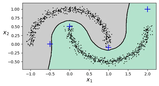
5. Các thuật toán phân cụm khác
Phân cụm Phổ (Spectral Clustering)
Sử dụng ma trận tương đồng (similarity matrix) giữa các điểm (thường là Affinity Matrix) và thực hiện phân tích phổ (eigenvalue decomposition) để giảm chiều dữ liệu trước khi phân cụm (thường dùng K-Means trong không gian mới).
from sklearn.cluster import SpectralClustering

sc1 = SpectralClustering(n_clusters=2, gamma=100, random_state=42)
sc1.fit(X)

sc2 = SpectralClustering(n_clusters=2, gamma=1, random_state=42)
sc2.fit(X)
output:
SpectralClustering(gamma=1, n_clusters=2, random_state=42)sc1.affinity_matrix_.round(2)output:
array([[1. , 0. , 0. , ..., 0. , 0. , 0. ],
[0. , 1. , 0.3, ..., 0. , 0. , 0. ],
[0. , 0.3, 1. , ..., 0. , 0. , 0. ],
...,
[0. , 0. , 0. , ..., 1. , 0. , 0. ],
[0. , 0. , 0. , ..., 0. , 1. , 0. ],
[0. , 0. , 0. , ..., 0. , 0. , 1. ]])# extra code – vẽ kết quả Spectral Clustering
def plot_spectral_clustering(sc, X, size, alpha, show_xlabels=True,
show_ylabels=True):
plt.scatter(X[:, 0], X[:, 1], marker='o', s=size, c='gray', alpha=alpha)
plt.scatter(X[:, 0], X[:, 1], marker='o', s=30, c='w')
plt.scatter(X[:, 0], X[:, 1], marker='.', s=10, c=sc.labels_, cmap="Paired")
if show_xlabels:
plt.xlabel("$x_1$")
else:
plt.tick_params(labelbottom=False)
if show_ylabels:
plt.ylabel("$x_2$", rotation=0)
else:
plt.tick_params(labelleft=False)
plt.title(f"RBF gamma={sc.gamma}")
plt.figure(figsize=(9, 3.2))
plt.subplot(121)
plot_spectral_clustering(sc1, X, size=500, alpha=0.1)
plt.subplot(122)
plot_spectral_clustering(sc2, X, size=4000, alpha=0.01, show_ylabels=False)
plt.show()
Phân cụm Phân cấp (Agglomerative Clustering)
Xây dựng cây phân cấp các cụm từ dưới lên (gom dần các cặp điểm gần nhất).
from sklearn.cluster import AgglomerativeClustering

X = np.array([0, 2, 5, 8.5]).reshape(-1, 1)
agg = AgglomerativeClustering(linkage="complete").fit(X)

def learned_parameters(estimator):
    return [attrib for attrib in dir(estimator)
            if attrib.endswith("_") and not attrib.startswith("_")]

learned_parameters(agg)
output:
['children_',
'labels_',
'n_clusters_',
'n_connected_components_',
'n_features_in_',
'n_leaves_']agg.children_output:
array([[0, 1],
[2, 3],
[4, 5]])6. Mô hình Hỗn hợp Gaussian (Gaussian Mixtures - GMM)
GMM là một mô hình xác suất giả định rằng các điểm dữ liệu được sinh ra từ một hỗn hợp của nhiều phân phối Gaussian (hình chuông) với các tham số chưa biết.
Khác với K-Means chỉ dùng tâm cụm, GMM mô hình hóa cụm bằng:
- Mean (): Tâm của phân phối.
- Covariance (): Hình dạng và độ rộng của phân phối (hình elip).
- Weight (): Tỷ trọng của cụm đó trong tổng thể.
# Tạo dữ liệu blobs méo mó (mà K-Means thất bại)
X1, y1 = make_blobs(n_samples=1000, centers=((4, -4), (0, 0)), random_state=42)
X1 = X1.dot(np.array([[0.374, 0.95], [0.732, 0.598]]))
X2, y2 = make_blobs(n_samples=250, centers=1, random_state=42)
X2 = X2 + [6, -8]
X = np.r_[X1, X2]
y = np.r_[y1, y2]
from sklearn.mixture import GaussianMixture
gm = GaussianMixture(n_components=3, n_init=10, random_state=42)
gm.fit(X)output:
GaussianMixture(n_components=3, n_init=10, random_state=42)Thuật toán Expectation-Maximization (EM) được dùng để tìm các tham số này.
# Trọng số của 3 cụm
gm.weights_
output:
array([0.40005972, 0.20961444, 0.39032584])# Tâm của 3 cụm
gm.means_output:
array([[-1.40764129, 1.42712848],
[ 3.39947665, 1.05931088],
[ 0.05145113, 0.07534576]])# Ma trận hiệp phương sai của 3 cụm
gm.covariances_output:
array([[[ 0.63478217, 0.72970097],
[ 0.72970097, 1.16094925]],
[[ 1.14740131, -0.03271106],
[-0.03271106, 0.95498333]],
[[ 0.68825143, 0.79617956],
[ 0.79617956, 1.21242183]]])gm.converged_output:
Truegm.n_iter_output:
4GMM cung cấp khả năng phân cụm mềm (xác suất thuộc về từng cụm) thông qua predict_proba().
gm.predict(X)output:
array([2, 2, 0, ..., 1, 1, 1])gm.predict_proba(X).round(3)output:
array([[0. , 0.023, 0.977],
[0.001, 0.016, 0.983],
[1. , 0. , 0. ],
...,
[0. , 1. , 0. ],
[0. , 1. , 0. ],
[0. , 1. , 0. ]])Mô hình tạo sinh (Generative Model)
Vì GMM mô hình hóa phân phối xác suất của dữ liệu (), nó có thể được dùng để sinh ra các mẫu dữ liệu mới trông giống như dữ liệu gốc.
X_new, y_new = gm.sample(6)
X_new
output:
array([[-2.32491052, 1.04752548],
[-1.16654983, 1.62795173],
[ 1.84860618, 2.07374016],
[ 3.98304484, 1.49869936],
[ 3.8163406 , 0.53038367],
[ 0.38079484, -0.56239369]])y_newoutput:
array([0, 0, 1, 1, 1, 2])Chúng ta cũng có thể ước lượng mật độ xác suất tại bất kỳ điểm nào bằng score_samples() (trả về log của mật độ).
gm.score_samples(X).round(2)output:
array([-2.61, -3.57, -3.33, ..., -3.51, -4.4 , -3.81])# extra code – kiểm tra tính hợp lệ của PDF (tổng tích phân = 1)
resolution = 100
grid = np.arange(-10, 10, 1 / resolution)
xx, yy = np.meshgrid(grid, grid)
X_full = np.vstack([xx.ravel(), yy.ravel()]).T
pdf = np.exp(gm.score_samples(X_full))
pdf_probas = pdf * (1 / resolution) ** 2
pdf_probas.sum()output:
np.float64(0.9999999999225088)Hình dưới đây hiển thị các đường đồng mức mật độ và ranh giới quyết định của GMM.
# extra code – tạo hình 8–16
from matplotlib.colors import LogNorm

def plot_gaussian_mixture(clusterer, X, resolution=1000, show_ylabels=True):
    mins = X.min(axis=0) - 0.1
    maxs = X.max(axis=0) + 0.1
    xx, yy = np.meshgrid(np.linspace(mins[0], maxs[0], resolution),
                         np.linspace(mins[1], maxs[1], resolution))
    Z = -clusterer.score_samples(np.c_[xx.ravel(), yy.ravel()])
    Z = Z.reshape(xx.shape)

    plt.contourf(xx, yy, Z,
                 norm=LogNorm(vmin=1.0, vmax=30.0),
                 levels=np.logspace(0, 2, 12))
    plt.contour(xx, yy, Z,
                norm=LogNorm(vmin=1.0, vmax=30.0),
                levels=np.logspace(0, 2, 12),
                linewidths=1, colors='k')

    Z = clusterer.predict(np.c_[xx.ravel(), yy.ravel()])
    Z = Z.reshape(xx.shape)
    plt.contour(xx, yy, Z,
                linewidths=2, colors='r', linestyles='dashed')

    plt.plot(X[:, 0], X[:, 1], 'k.', markersize=2)
    plot_centroids(clusterer.means_, clusterer.weights_)

    plt.xlabel("$x_1$")
    if show_ylabels:
        plt.ylabel("$x_2$", rotation=0)
    else:
        plt.tick_params(labelleft=False)

plt.figure(figsize=(8, 4))
plot_gaussian_mixture(gm, X)
plt.show()
Các loại ma trận hiệp phương sai (covariance_type)
Bạn có thể ràng buộc hình dạng của các cụm để giảm số lượng tham số cần học:
"spherical": Cụm hình cầu."diag": Cụm hình elip nhưng trục song song với trục tọa độ."tied": Tất cả các cụm có cùng hình dạng elip."full": (Mặc định) Cụm có hình elip tùy ý.
# extra code – tạo hình 8–17 so sánh các loại covariance
gm_full = GaussianMixture(n_components=3, n_init=10,
                          covariance_type="full", random_state=42)
gm_tied = GaussianMixture(n_components=3, n_init=10,
                          covariance_type="tied", random_state=42)
gm_spherical = GaussianMixture(n_components=3, n_init=10,
                               covariance_type="spherical", random_state=42)
gm_diag = GaussianMixture(n_components=3, n_init=10,
                          covariance_type="diag", random_state=42)
gm_full.fit(X)
gm_tied.fit(X)
gm_spherical.fit(X)
gm_diag.fit(X)

def compare_gaussian_mixtures(gm1, gm2, X):
    plt.figure(figsize=(9, 4))

    plt.subplot(121)
    plot_gaussian_mixture(gm1, X)
    plt.title(f'covariance_type="{gm1.covariance_type}"')

    plt.subplot(122)
    plot_gaussian_mixture(gm2, X, show_ylabels=False)
    plt.title(f'covariance_type="{gm2.covariance_type}"')

compare_gaussian_mixtures(gm_tied, gm_spherical, X)
plt.show()
# extra code – so sánh full và diag
compare_gaussian_mixtures(gm_full, gm_diag, X)
plt.tight_layout()
plt.show()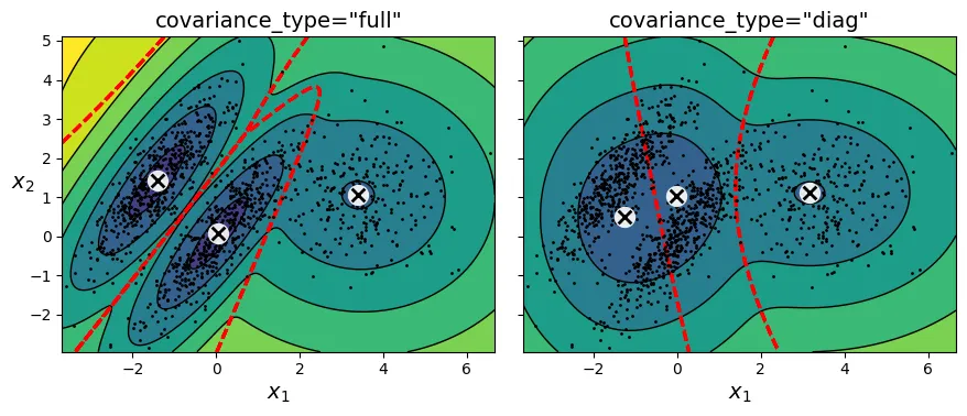
Phát hiện bất thường (Anomaly Detection) với GMM
Các điểm dữ liệu nằm trong vùng có mật độ thấp có thể được coi là bất thường. Chúng ta xác định ngưỡng mật độ (ví dụ: 2% thấp nhất) và coi tất cả các điểm dưới ngưỡng này là ngoại lai.
densities = gm.score_samples(X)
density_threshold = np.percentile(densities, 2)
anomalies = X[densities < density_threshold]
# extra code – tạo hình 8–18 đánh dấu các điểm bất thường
plt.figure(figsize=(8, 4))
plot_gaussian_mixture(gm, X)
plt.scatter(anomalies[:, 0], anomalies[:, 1], color='r', marker='*')
plt.ylim(top=5.1)
plt.show()
Lựa chọn số lượng cụm ()
Với GMM, chúng ta dùng BIC (Bayesian Information Criterion) hoặc AIC (Akaike Information Criterion). Cả hai chỉ số này đều phạt các mô hình phức tạp (nhiều tham số) và thưởng các mô hình khớp dữ liệu tốt (likelihood cao).
Giá trị BIC/AIC càng thấp càng tốt.
# extra code – tạo hình 8–19 giải thích BIC/AIC
from scipy.stats import norm

x_val = 2.5
std_val = 1.3
x_range = [-6, 4]
x_proba_range = [-2, 2]
stds_range = [1, 2]

xs = np.linspace(x_range[0], x_range[1], 501)
stds = np.linspace(stds_range[0], stds_range[1], 501)
Xs, Stds = np.meshgrid(xs, stds)
Z = 2 * norm.pdf(Xs - 1.0, 0, Stds) + norm.pdf(Xs + 4.0, 0, Stds)
Z = Z / Z.sum(axis=1)[:, np.newaxis] / (xs[1] - xs[0])

x_example_idx = (xs >= x_val).argmax()
max_idx = Z[:, x_example_idx].argmax()
max_val = Z[:, x_example_idx].max()
s_example_idx = (stds >= std_val).argmax()

x_range_min_idx = (xs >= x_proba_range[0]).argmax()
x_range_max_idx = (xs >= x_proba_range[1]).argmax()

log_max_idx = np.log(Z[:, x_example_idx]).argmax()
log_max_val = np.log(Z[:, x_example_idx]).max()

plt.figure(figsize=(8, 4.5))

plt.subplot(2, 2, 1)
plt.contourf(Xs, Stds, Z, cmap="GnBu")
plt.plot([-6, 4], [std_val, std_val], "k-", linewidth=2)
plt.plot([x_val, x_val], [1, 2], "b-", linewidth=2)
plt.ylabel(r"$\theta$", rotation=0, labelpad=10)
plt.title(r"Model $f(x; \theta)$")

plt.subplot(2, 2, 2)
plt.plot(stds, Z[:, x_example_idx], "b-")
plt.plot(stds[max_idx], max_val, "r.")
plt.plot([stds[max_idx], stds[max_idx]], [0, max_val], "r:")
plt.plot([0, stds[max_idx]], [max_val, max_val], "r:")
plt.text(stds[max_idx]+ 0.01, 0.081, r"$\hat{\theta}$")
plt.text(stds[max_idx]+ 0.01, max_val - 0.006, r"$Max$")
plt.text(1.01, max_val - 0.008, r"$\hat{\mathcal{L}}$")
plt.ylabel(r"$\mathcal{L}$", rotation=0, labelpad=10)
plt.title(fr"$\mathcal{{L}}(\theta|x={x_val}) = f(x={x_val}; \theta)$")
plt.grid()
plt.axis([1, 2, 0.08, 0.12])

plt.subplot(2, 2, 3)
plt.plot(xs, Z[s_example_idx], "k-")
plt.fill_between(xs[x_range_min_idx:x_range_max_idx+1],
                 Z[s_example_idx, x_range_min_idx:x_range_max_idx+1], alpha=0.2)
plt.xlabel(r"$x$")
plt.ylabel("PDF")
plt.title(fr"PDF $f(x; \theta={std_val})$")
plt.grid()
plt.axis([-6, 4, 0, 0.25])

plt.subplot(2, 2, 4)
plt.plot(stds, np.log(Z[:, x_example_idx]), "b-")
plt.plot(stds[log_max_idx], log_max_val, "r.")
plt.plot([stds[log_max_idx], stds[log_max_idx]], [-5, log_max_val], "r:")
plt.plot([0, stds[log_max_idx]], [log_max_val, log_max_val], "r:")
plt.text(stds[log_max_idx]+ 0.01, log_max_val - 0.06, r"$Max$")
plt.text(stds[log_max_idx]+ 0.01, -2.49, r"$\hat{\theta}$")
plt.text(1.01, log_max_val - 0.08, r"$\log \, \hat{\mathcal{L}}$")
plt.xlabel(r"$\theta$")
plt.ylabel(r"$\log\mathcal{L}$", rotation=0, labelpad=10)
plt.title(fr"$\log \, \mathcal{{L}}(\theta|x={x_val})$")
plt.grid()
plt.axis([1, 2, -2.5, -2.1])

plt.show()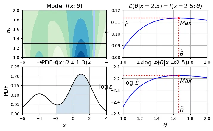
gm.bic(X)output:
8189.733705221636gm.aic(X)output:
8102.508425106598# extra code – tính BIC/AIC thủ công
n_clusters = 3
n_dims = 2
n_params_for_weights = n_clusters - 1
n_params_for_means = n_clusters * n_dims
n_params_for_covariance = n_clusters * n_dims * (n_dims + 1) // 2
n_params = n_params_for_weights + n_params_for_means + n_params_for_covariance
max_log_likelihood = gm.score(X) * len(X) # log(L^)
bic = np.log(len(X)) * n_params - 2 * max_log_likelihood
aic = 2 * n_params - 2 * max_log_likelihood
print(f"bic = {bic}")
print(f"aic = {aic}")
print(f"n_params = {n_params}")output:
bic = 8189.733705221636
aic = 8102.508425106598
n_params = 17# extra code – tạo hình 8–20 biểu đồ BIC/AIC theo k
gms_per_k = [GaussianMixture(n_components=k, n_init=10, random_state=42).fit(X)
for k in range(1, 11)]
bics = [model.bic(X) for model in gms_per_k]
aics = [model.aic(X) for model in gms_per_k]
plt.figure(figsize=(8, 3))
plt.plot(range(1, 11), bics, "bo-", label="BIC")
plt.plot(range(1, 11), aics, "go--", label="AIC")
plt.xlabel("$k$")
plt.ylabel("Information Criterion")
plt.axis([1, 9.5, min(aics) - 50, max(aics) + 50])
plt.annotate("", xy=(3, bics[2]), xytext=(3.4, 8650),
arrowprops=dict(facecolor='black', shrink=0.1))
plt.text(3.5, 8660, "Minimum", horizontalalignment="center")
plt.legend()
plt.grid()
plt.show()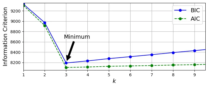
Mô hình Hỗn hợp Gaussian Bayes (Bayesian Gaussian Mixture)
Nếu bạn không muốn dò tìm , hãy dùng BayesianGaussianMixture. Nó sử dụng phân phối Dirichlet Process để tự động loại bỏ các cụm thừa (trọng số về 0).
from sklearn.mixture import BayesianGaussianMixture

# Đặt k=10, lớn hơn số cụm thực tế là 3
bgm = BayesianGaussianMixture(n_components=10, n_init=10, max_iter=500,
                              random_state=42)
bgm.fit(X)
bgm.weights_.round(2)
output:
array([0.4 , 0.21, 0.39, 0. , 0. , 0. , 0. , 0. , 0. , 0. ])Kết quả cho thấy chỉ có 3 trọng số là đáng kể.
# extra code – vẽ kết quả của Bayesian GMM
plt.figure(figsize=(8, 5))
plot_gaussian_mixture(bgm, X)
plt.show()
# extra code – tạo hình 8–21 GMM trên dữ liệu moons
X_moons, y_moons = make_moons(n_samples=1000, noise=0.05, random_state=42)
bgm = BayesianGaussianMixture(n_components=10, n_init=10, max_iter=500, random_state=42)
bgm.fit(X_moons)

plt.figure(figsize=(9, 3.2))

plt.subplot(121)
plot_data(X_moons)
plt.xlabel("$x_1$")
plt.ylabel("$x_2$", rotation=0)
plt.grid()

plt.subplot(122)
plot_gaussian_mixture(bgm, X_moons, show_ylabels=False)
plt.show()
7. Bài tập thực hành: Bộ dữ liệu khuôn mặt Olivetti
Chuẩn bị dữ liệu
import os
import urllib.request
from sklearn.datasets import fetch_olivetti_faces

# 1. Define the path. Scikit-learn looks in the root of data_home for this specific file.
data_home = os.path.expanduser("~/scikit_learn_data")
if not os.path.exists(data_home):
    os.makedirs(data_home)

# 2. Define the working URL (Mirror) and target path
url = "https://github.com/probml/pmtk3/raw/master/bigData/olivettiFaces/olivettiFaces.mat"
target_path = os.path.join(data_home, "olivettifaces.mat")

# 3. Download the file manually
if not os.path.exists(target_path):
    print(f"Downloading to {target_path}...")
    try:
        urllib.request.urlretrieve(url, target_path)
        print("Download successful!")
    except Exception as e:
        print(f"Failed to download: {e}")
else:
    print(f"File already exists at {target_path}")

# 4. Load the dataset
# Scikit-learn will see the local file and skip the broken Figshare download
try:
    olivetti = fetch_olivetti_faces()
    print(f"\nSuccess! Dataset loaded: {olivetti.images.shape}")
except Exception as e:
    print(f"\nError loading dataset: {e}")
output:
Downloading to /root/scikit_learn_data/olivettifaces.mat...
Download successful!
downloading Olivetti faces from https://ndownloader.figshare.com/files/5976027 to /root/scikit_learn_data
Success! Dataset loaded: (400, 64, 64)olivetti.targetoutput:
array([ 0, 0, 0, 0, 0, 0, 0, 0, 0, 0, 1, 1, 1, 1, 1, 1, 1,
1, 1, 1, 2, 2, 2, 2, 2, 2, 2, 2, 2, 2, 3, 3, 3, 3,
3, 3, 3, 3, 3, 3, 4, 4, 4, 4, 4, 4, 4, 4, 4, 4, 5,
5, 5, 5, 5, 5, 5, 5, 5, 5, 6, 6, 6, 6, 6, 6, 6, 6,
6, 6, 7, 7, 7, 7, 7, 7, 7, 7, 7, 7, 8, 8, 8, 8, 8,
8, 8, 8, 8, 8, 9, 9, 9, 9, 9, 9, 9, 9, 9, 9, 10, 10,
10, 10, 10, 10, 10, 10, 10, 10, 11, 11, 11, 11, 11, 11, 11, 11, 11,
11, 12, 12, 12, 12, 12, 12, 12, 12, 12, 12, 13, 13, 13, 13, 13, 13,
13, 13, 13, 13, 14, 14, 14, 14, 14, 14, 14, 14, 14, 14, 15, 15, 15,
15, 15, 15, 15, 15, 15, 15, 16, 16, 16, 16, 16, 16, 16, 16, 16, 16,
17, 17, 17, 17, 17, 17, 17, 17, 17, 17, 18, 18, 18, 18, 18, 18, 18,
18, 18, 18, 19, 19, 19, 19, 19, 19, 19, 19, 19, 19, 20, 20, 20, 20,
20, 20, 20, 20, 20, 20, 21, 21, 21, 21, 21, 21, 21, 21, 21, 21, 22,
22, 22, 22, 22, 22, 22, 22, 22, 22, 23, 23, 23, 23, 23, 23, 23, 23,
23, 23, 24, 24, 24, 24, 24, 24, 24, 24, 24, 24, 25, 25, 25, 25, 25,
25, 25, 25, 25, 25, 26, 26, 26, 26, 26, 26, 26, 26, 26, 26, 27, 27,
27, 27, 27, 27, 27, 27, 27, 27, 28, 28, 28, 28, 28, 28, 28, 28, 28,
28, 29, 29, 29, 29, 29, 29, 29, 29, 29, 29, 30, 30, 30, 30, 30, 30,
30, 30, 30, 30, 31, 31, 31, 31, 31, 31, 31, 31, 31, 31, 32, 32, 32,
32, 32, 32, 32, 32, 32, 32, 33, 33, 33, 33, 33, 33, 33, 33, 33, 33,
34, 34, 34, 34, 34, 34, 34, 34, 34, 34, 35, 35, 35, 35, 35, 35, 35,
35, 35, 35, 36, 36, 36, 36, 36, 36, 36, 36, 36, 36, 37, 37, 37, 37,
37, 37, 37, 37, 37, 37, 38, 38, 38, 38, 38, 38, 38, 38, 38, 38, 39,
39, 39, 39, 39, 39, 39, 39, 39, 39])from sklearn.model_selection import StratifiedShuffleSplit
strat_split = StratifiedShuffleSplit(n_splits=1, test_size=40, random_state=42)
train_valid_idx, test_idx = next(strat_split.split(olivetti.data,
olivetti.target))
X_train_valid = olivetti.data[train_valid_idx]
y_train_valid = olivetti.target[train_valid_idx]
X_test = olivetti.data[test_idx]
y_test = olivetti.target[test_idx]
strat_split = StratifiedShuffleSplit(n_splits=1, test_size=80, random_state=43)
train_idx, valid_idx = next(strat_split.split(X_train_valid, y_train_valid))
X_train = X_train_valid[train_idx]
y_train = y_train_valid[train_idx]
X_valid = X_train_valid[valid_idx]
y_valid = y_train_valid[valid_idx]
print(X_train.shape, y_train.shape)
print(X_valid.shape, y_valid.shape)
print(X_test.shape, y_test.shape)output:
(280, 4096) (280,)
(80, 4096) (80,)
(40, 4096) (40,)Giảm chiều dữ liệu bằng PCA (giữ lại 99% phương sai).
from sklearn.decomposition import PCA

pca = PCA(0.99)
X_train_pca = pca.fit_transform(X_train)
X_valid_pca = pca.transform(X_valid)
X_test_pca = pca.transform(X_test)
pca.n_components_
output:
np.int64(199)Phân cụm khuôn mặt với K-Means
Sử dụng Silhouette Score để tìm tối ưu.
from sklearn.cluster import KMeans

k_range = range(5, 150, 5)
kmeans_per_k = []
for k in k_range:
    print(f"k={k}")
    kmeans = KMeans(n_clusters=k, random_state=42)
    kmeans.fit(X_train_pca)
    kmeans_per_k.append(kmeans)
output:
k=5
k=10
k=15
k=20
k=25
k=30
k=35
k=40
k=45
k=50
k=55
k=60
k=65
k=70
k=75
k=80
k=85
k=90
k=95
k=100
k=105
k=110
k=115
k=120
k=125
k=130
k=135
k=140
k=145from sklearn.metrics import silhouette_score
silhouette_scores = [silhouette_score(X_train_pca, model.labels_)
for model in kmeans_per_k]
best_index = np.argmax(silhouette_scores)
best_k = k_range[best_index]
best_score = silhouette_scores[best_index]
plt.figure(figsize=(8, 3))
plt.plot(k_range, silhouette_scores, "bo-")
plt.xlabel("$k$")
plt.ylabel("Silhouette score")
plt.plot(best_k, best_score, "rs")
plt.grid()
plt.show()
best_koutput:
75inertias = [model.inertia_ for model in kmeans_per_k]
best_inertia = inertias[best_index]
plt.figure(figsize=(8, 3.5))
plt.plot(k_range, inertias, "bo-")
plt.xlabel("$k$")
plt.ylabel("Inertia")
plt.plot(best_k, best_inertia, "rs")
plt.grid()
plt.show()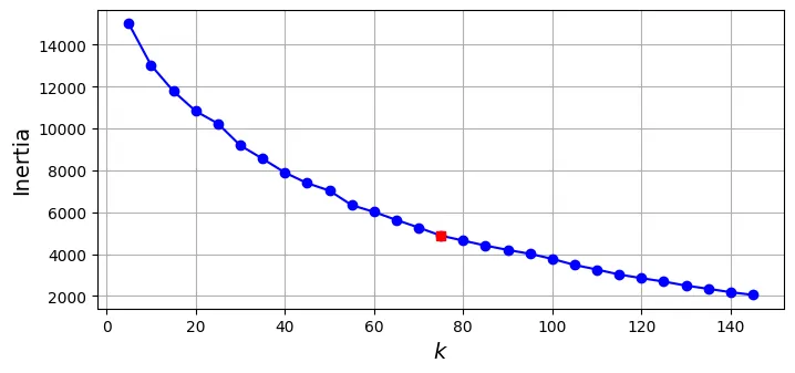
best_model = kmeans_per_k[best_index]# Hàm vẽ các khuôn mặt
def plot_faces(faces, labels, n_cols=5):
faces = faces.reshape(-1, 64, 64)
n_rows = (len(faces) - 1) // n_cols + 1
plt.figure(figsize=(n_cols, n_rows * 1.1))
for index, (face, label) in enumerate(zip(faces, labels)):
plt.subplot(n_rows, n_cols, index + 1)
plt.imshow(face, cmap="gray")
plt.axis("off")
plt.title(label)
plt.show()
for cluster_id in np.unique(best_model.labels_):
print("Cluster", cluster_id)
in_cluster = best_model.labels_==cluster_id
faces = X_train[in_cluster]
labels = y_train[in_cluster]
plot_faces(faces, labels)output:
Cluster 0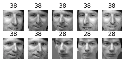
output:
Cluster 1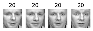
output:
Cluster 2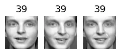
output:
Cluster 3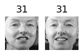
output:
Cluster 4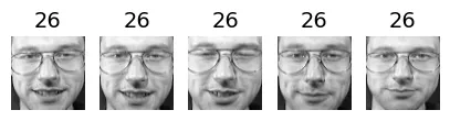
output:
Cluster 5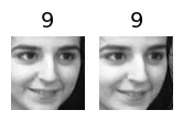
output:
Cluster 6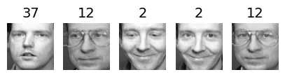
output:
Cluster 7
output:
Cluster 8
output:
Cluster 9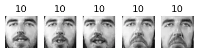
output:
Cluster 10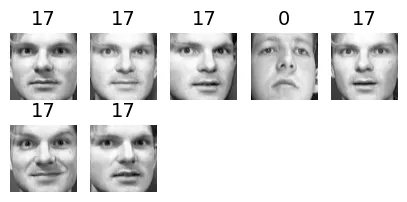
output:
Cluster 11
output:
Cluster 12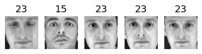
output:
Cluster 13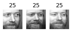
output:
Cluster 14
output:
Cluster 15
output:
Cluster 16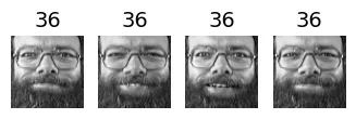
output:
Cluster 17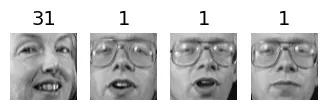
output:
Cluster 18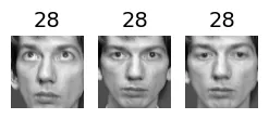
output:
Cluster 19
output:
Cluster 20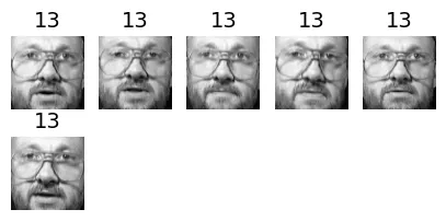
output:
Cluster 21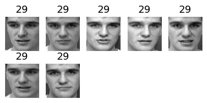
output:
Cluster 22
output:
Cluster 23
output:
Cluster 24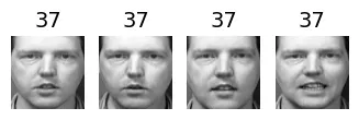
output:
Cluster 25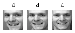
output:
Cluster 26
output:
Cluster 27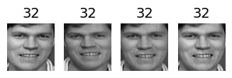
output:
Cluster 28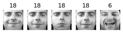
output:
Cluster 29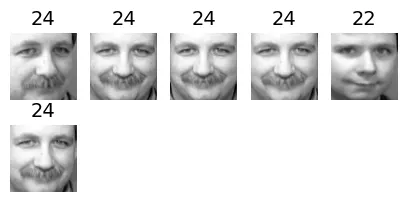
output:
Cluster 30
output:
Cluster 31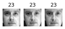
output:
Cluster 32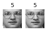
output:
Cluster 33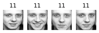
output:
Cluster 34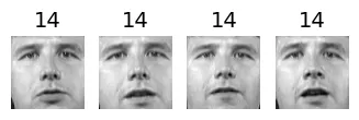
output:
Cluster 35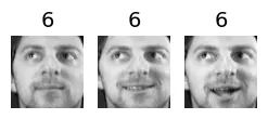
output:
Cluster 36
output:
Cluster 37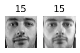
output:
Cluster 38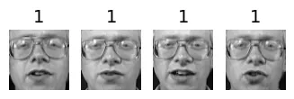
output:
Cluster 39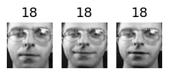
output:
Cluster 40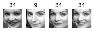
output:
Cluster 41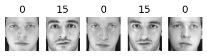
output:
Cluster 42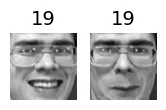
output:
Cluster 43
output:
Cluster 44
output:
Cluster 45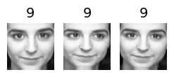
output:
Cluster 46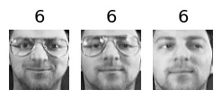
output:
Cluster 47
output:
Cluster 48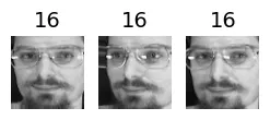
output:
Cluster 49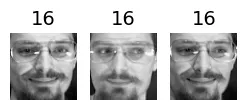
output:
Cluster 50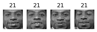
output:
Cluster 51
output:
Cluster 52
output:
Cluster 53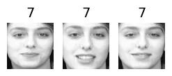
output:
Cluster 54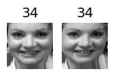
output:
Cluster 55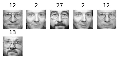
output:
Cluster 56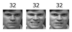
output:
Cluster 57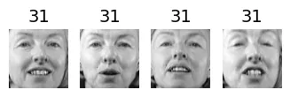
output:
Cluster 58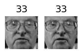
output:
Cluster 59
output:
Cluster 60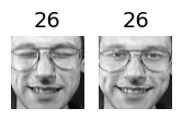
output:
Cluster 61
output:
Cluster 62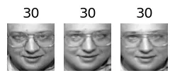
output:
Cluster 63
output:
Cluster 64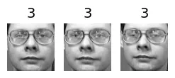
output:
Cluster 65
output:
Cluster 66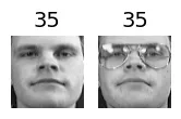
output:
Cluster 67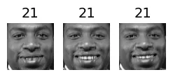
output:
Cluster 68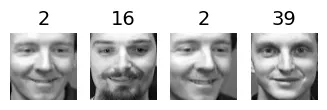
output:
Cluster 69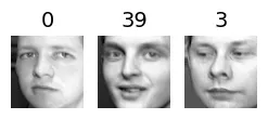
output:
Cluster 70
output:
Cluster 71
output:
Cluster 72
output:
Cluster 73
output:
Cluster 74
Sử dụng Phân cụm để tiền xử lý cho Phân loại
# Huấn luyện Random Forest trên dữ liệu gốc (đã qua PCA)
from sklearn.ensemble import RandomForestClassifier
clf = RandomForestClassifier(n_estimators=150, random_state=42)
clf.fit(X_train_pca, y_train)
clf.score(X_valid_pca, y_valid)output:
0.9375# Huấn luyện trên dữ liệu đã giảm chiều bằng K-Means
X_train_reduced = best_model.transform(X_train_pca)
X_valid_reduced = best_model.transform(X_valid_pca)
X_test_reduced = best_model.transform(X_test_pca)
clf = RandomForestClassifier(n_estimators=150, random_state=42)
clf.fit(X_train_reduced, y_train)
clf.score(X_valid_reduced, y_valid)output:
0.7375from sklearn.pipeline import make_pipeline
for n_clusters in k_range:
pipeline = make_pipeline(
KMeans(n_clusters=n_clusters, random_state=42),
RandomForestClassifier(n_estimators=150, random_state=42)
)
pipeline.fit(X_train_pca, y_train)
print(n_clusters, pipeline.score(X_valid_pca, y_valid))output:
5 0.4
10 0.4375
15 0.5875
20 0.6
25 0.6625
30 0.6625
35 0.6625
40 0.675
45 0.6625
50 0.6875
55 0.75
60 0.6875
65 0.725
70 0.7
75 0.7375
80 0.725
85 0.7625
90 0.775
95 0.775
100 0.7625
105 0.75
110 0.725
115 0.7625
120 0.7625
125 0.7375
130 0.7375
135 0.725
140 0.8
145 0.725X_train_extended = np.c_[X_train_pca, X_train_reduced]
X_valid_extended = np.c_[X_valid_pca, X_valid_reduced]
X_test_extended = np.c_[X_test_pca, X_test_reduced]
clf = RandomForestClassifier(n_estimators=150, random_state=42)
clf.fit(X_train_extended, y_train)
clf.score(X_valid_extended, y_valid)output:
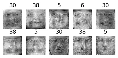
0.85GMM: Sinh khuôn mặt mới và Phát hiện bất thường
from sklearn.mixture import GaussianMixture
gm = GaussianMixture(n_components=40, random_state=42)
y_pred = gm.fit_predict(X_train_pca)# Sinh 20 khuôn mặt mới
n_gen_faces = 20
gen_faces_reduced, y_gen_faces = gm.sample(n_samples=n_gen_faces)
gen_faces = pca.inverse_transform(gen_faces_reduced)
plot_faces(gen_faces, y_gen_faces)output:
/usr/local/lib/python3.12/dist-packages/sklearn/mixture/_base.py:468: RuntimeWarning: covariance is not symmetric positive-semidefinite.
rng.multivariate_normal(mean, covariance, int(sample))
n_rotated = 4
rotated = np.transpose(X_train[:n_rotated].reshape(-1, 64, 64), axes=[0, 2, 1])
rotated = rotated.reshape(-1, 64*64)
y_rotated = y_train[:n_rotated]
n_flipped = 3
flipped = X_train[:n_flipped].reshape(-1, 64, 64)[:, ::-1]
flipped = flipped.reshape(-1, 64*64)
y_flipped = y_train[:n_flipped]
n_darkened = 3
darkened = X_train[:n_darkened].copy()
darkened[:, 1:-1] *= 0.3
y_darkened = y_train[:n_darkened]
X_bad_faces = np.r_[rotated, flipped, darkened]
y_bad = np.concatenate([y_rotated, y_flipped, y_darkened])
plot_faces(X_bad_faces, y_bad)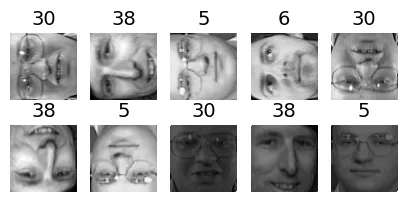
X_bad_faces_pca = pca.transform(X_bad_faces)
gm.score_samples(X_bad_faces_pca)output:
array([-19610904., -17223394., -41810812., -50242452., -32037220.,
-13569778., -29925510., -87415344., -97655488., -51947340.],
dtype=float32)gm.score_samples(X_train_pca[:10])output:
array([1162.6652, 1111.7946, 1156.0321, 1170.4318, 1073.5156, 1139.5026,
1113.5194, 1073.5156, 1048.4954, 1048.4954], dtype=float32)Sử dụng PCA để phát hiện bất thường
X_train_pca.round(2)output:
array([[ -3.78, 1.85, -5.14, ..., 0.14, -0.21, 0.06],
[-10.15, 1.53, -0.77, ..., -0.12, -0.14, -0.02],
[ 10.02, -2.88, -0.92, ..., -0.07, -0. , 0.12],
...,
[ -2.48, -2.96, 1.3 , ..., 0.02, 0.03, -0.15],
[ 3.22, -5.35, 1.39, ..., -0.06, -0.23, 0.16],
[ 0.92, 3.65, 2.26, ..., -0.14, -0.07, 0.06]],
dtype=float32)def reconstruction_errors(pca, X):
X_pca = pca.transform(X)
X_reconstructed = pca.inverse_transform(X_pca)
mse = np.square(X_reconstructed - X).mean(axis=-1)
return mse# Sai số tái tạo trung bình của ảnh thật
reconstruction_errors(pca, X_train).mean()output:
np.float32(0.00019205351)# Sai số tái tạo trung bình của ảnh lỗi (lớn hơn nhiều)
reconstruction_errors(pca, X_bad_faces).mean()output:
np.float32(0.004707354)plot_faces(X_bad_faces, y_bad)
X_bad_faces_reconstructed = pca.inverse_transform(X_bad_faces_pca)
plot_faces(X_bad_faces_reconstructed, y_bad)