[ML101] Chương 6: Học kết hợp và Rừng ngẫu nhiên
Ensemble Learning, Random Forests và các phương pháp boosting
Bài viết có tham khảo, sử dụng và sửa đổi tài nguyên từ kho lưu trữ handson-mlp, tuân thủ giấy phép Apache‑2.0. Chúng tôi chân thành cảm ơn tác giả Aurélien Géron (@aureliengeron) vì sự chia sẻ kiến thức tuyệt vời và những đóng góp quý giá cho cộng đồng.
Chào mừng bạn đến với Chương 6. Trong chương này, chúng ta sẽ khám phá một trong những kỹ thuật mạnh mẽ trong Học máy (Machine Learning): Học kết hợp (Ensemble Learning).
Ý tưởng cốt lõi của Học kết hợp dựa trên nguyên lý “trí tuệ đám đông” (wisdom of the crowd). Về mặt toán học, điều này liên quan đến định lý về sự hội tụ của các biến ngẫu nhiên độc lập. Thay vì phụ thuộc vào một mô hình duy nhất (ví dụ: một Cây quyết định), chúng ta tập hợp một nhóm các mô hình dự đoán lại với nhau. Nếu các mô hình này mắc các lỗi không tương quan (uncorrelated errors), việc kết hợp chúng sẽ giảm phương sai tổng thể và cải thiện độ chính xác dự đoán.
Chúng ta cũng sẽ tìm hiểu về Rừng ngẫu nhiên (Random Forests), một thuật toán Học kết hợp phổ biến dựa trên Cây quyết định, cũng như các kỹ thuật Boosting (Tăng cường) và Stacking (Xếp chồng).
Bạn có thể chạy trực tiếp các đoạn mã code tại: Google Colab.
Cài đặt môi trường
Trước khi đi vào chi tiết, như thường lệ, chúng ta cần đảm bảo môi trường Python đáp ứng các yêu cầu về phiên bản. Dự án này yêu cầu Python 3.10 trở lên và Scikit-Learn phiên bản 1.6.1 trở lên.
# Kiểm tra phiên bản Python
import sys
assert sys.version_info >= (3, 10)

# Kiểm tra phiên bản Scikit-Learn
from packaging.version import Version
import sklearn
assert Version(sklearn.__version__) >= Version("1.6.1")
Như thường lệ, chúng ta sẽ thiết lập kích thước phông chữ mặc định cho thư viện matplotlib để các biểu đồ hiển thị rõ ràng và đẹp mắt hơn.
import matplotlib.pyplot as plt

# Thiết lập kích thước phông chữ và các thành phần biểu đồ
plt.rc('font', size=14)
plt.rc('axes', labelsize=14, titlesize=14)
plt.rc('legend', fontsize=14)
plt.rc('xtick', labelsize=10)
plt.rc('ytick', labelsize=10)
1. Bộ phân loại biểu quyết (Voting Classifiers)
Hãy bắt đầu với hình thức học kết hợp đơn giản nhất: Biểu quyết (Voting).
Cơ sở lý thuyết của phương pháp này dựa trên Luật số lớn (Law of Large Numbers). Giả sử bạn có một đồng xu hơi lệch, với xác suất ra mặt ngửa là . Nếu bạn tung nó lần, xác suất để tỷ lệ mặt ngửa lớn hơn 50% sẽ tăng lên khi tăng.
Cụ thể, nếu là biến ngẫu nhiên Bernoulli đại diện cho lần tung thứ , thì tổng số mặt ngửa sẽ tuân theo phân phối nhị thức. Khi , theo định lý giới hạn trung tâm, phân phối của tỷ lệ sẽ hội tụ về kỳ vọng với phương sai tiến về 0.
Đoạn mã dưới đây mô phỏng việc tung đồng xu 10.000 lần cho 10 thí nghiệm khác nhau để minh họa sự hội tụ này.
# extra code – ô này tạo ra Hình 6–3 minh họa Luật số lớn
import matplotlib.pyplot as plt
import numpy as np

heads_proba = 0.51  # Xác suất mặt ngửa là 51%
rng = np.random.default_rng(seed=42)

# Mô phỏng 10.000 lần tung đồng xu cho 10 thí nghiệm
coin_tosses = (rng.random((10000, 10)) < heads_proba).astype(np.int32)

# Tính tổng tích lũy số lần mặt ngửa
cumulative_heads = coin_tosses.cumsum(axis=0)

# Tính tỷ lệ mặt ngửa tích lũy
cumulative_heads_ratio = cumulative_heads / np.arange(1, 10001).reshape(-1, 1)

# Vẽ biểu đồ
plt.figure(figsize=(8, 3.5))
plt.plot(cumulative_heads_ratio)
plt.plot([0, 10000], [0.51, 0.51], "k--", linewidth=2, label="51%")
plt.plot([0, 10000], [0.5, 0.5], "k-", label="50%")
plt.xlabel("Number of coin tosses")
plt.ylabel("Heads ratio")
plt.legend(loc="lower right")
plt.axis([0, 10000, 0.42, 0.58])
plt.grid()
plt.show()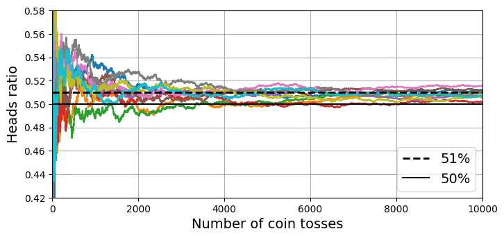
Tiếp theo, chúng ta sẽ xây dựng một bộ phân loại biểu quyết thực sự bằng cách sử dụng tập dữ liệu moons. Chúng ta sẽ kết hợp ba mô hình khác nhau: Hồi quy Logistic (Logistic Regression), Rừng ngẫu nhiên (Random Forest) và Máy vector hỗ trợ (SVM).
Trong Hard Voting (Biểu quyết cứng), mỗi bộ phân loại sẽ đưa ra một dự đoán lớp . Lớp dự đoán cuối cùng là lớp nhận được đa số phiếu bầu (mode):
from sklearn.datasets import make_moons
from sklearn.ensemble import RandomForestClassifier, VotingClassifier
from sklearn.linear_model import LogisticRegression
from sklearn.model_selection import train_test_split
from sklearn.svm import SVC

# Tạo dữ liệu moons
X, y = make_moons(n_samples=500, noise=0.30, random_state=42)
X_train, X_test, y_train, y_test = train_test_split(X, y, random_state=42)

# Khởi tạo bộ phân loại biểu quyết với 3 mô hình con
voting_clf = VotingClassifier(
    estimators=[
        ('lr', LogisticRegression(random_state=42)),
        ('rf', RandomForestClassifier(random_state=42)),
        ('svc', SVC(random_state=42))
    ])

# Huấn luyện mô hình
voting_clf.fit(X_train, y_train)
output:
VotingClassifier(estimators=[('lr', LogisticRegression(random_state=42)),
('rf', RandomForestClassifier(random_state=42)),
('svc', SVC(random_state=42))])Sau khi huấn luyện, chúng ta hãy xem độ chính xác của từng mô hình riêng lẻ trên tập kiểm tra (test set).
for name, clf in voting_clf.named_estimators_.items():
    print(name, "=", clf.score(X_test, y_test))
output:
lr = 0.864
rf = 0.896
svc = 0.896Bây giờ, hãy xem dự đoán của mô hình biểu quyết cho mẫu đầu tiên trong tập kiểm tra.
voting_clf.predict(X_test[:1])output:
array([1])Để hiểu rõ hơn, chúng ta có thể xem dự đoán riêng lẻ của từng mô hình thành viên:
[clf.predict(X_test[:1]) for clf in voting_clf.estimators_]output:
[array([1]), array([1]), array([0])]Cuối cùng, hãy kiểm tra độ chính xác tổng thể của bộ phân loại biểu quyết. Thông thường, nó sẽ cao hơn độ chính xác của các mô hình thành phần.
voting_clf.score(X_test, y_test)output:
0.912Soft Voting (Biểu quyết mềm)
Nếu tất cả các bộ phân loại đều có thể ước tính xác suất của từng lớp (có phương thức predict_proba()), chúng ta có thể sử dụng Soft Voting. Trong phương pháp này, chúng ta tính trung bình xác suất của từng lớp trên tất cả các bộ phân loại và chọn lớp có xác suất trung bình cao nhất.
Soft Voting thường cho kết quả tốt hơn Hard Voting vì nó cân nhắc đến mức độ tự tin (confidence) của từng mô hình.
Lưu ý: Mô hình SVC mặc định không tính xác suất, nên ta phải đặt tham số probability=True. Điều này sẽ kích hoạt việc sử dụng Cross-Validation 5-fold để hiệu chuẩn xác suất (dùng Platt scaling), làm chậm quá trình huấn luyện nhưng cho phép dự đoán xác suất.
# Chuyển sang chế độ soft voting
voting_clf.voting = "soft"

# Cấu hình lại SVC để hỗ trợ tính xác suất
voting_clf.named_estimators["svc"].probability = True

# Huấn luyện lại và đánh giá
voting_clf.fit(X_train, y_train)
voting_clf.score(X_test, y_test)
output:
0.922. Bagging và Pasting
Thay vì sử dụng các thuật toán khác nhau, một cách tiếp cận khác là sử dụng cùng một thuật toán nhưng huấn luyện trên các tập con ngẫu nhiên khác nhau của dữ liệu huấn luyện.
- Bagging (Bootstrap Aggregating): Lấy mẫu có hoàn lại (sampling with replacement). Cùng một mẫu dữ liệu có thể xuất hiện nhiều lần trong một tập con huấn luyện.
- Pasting: Lấy mẫu không hoàn lại (sampling without replacement).
Cả hai phương pháp đều giúp giảm phương sai (variance) của mô hình mà không làm tăng đáng kể độ lệch (bias).
Dưới đây, chúng ta sử dụng BaggingClassifier của Scikit-Learn với 500 cây quyết định. Tham số max_samples=100 nghĩa là mỗi cây được huấn luyện trên 100 mẫu được chọn ngẫu nhiên. bootstrap=True (mặc định) kích hoạt Bagging; nếu False thì là Pasting.
from sklearn.ensemble import BaggingClassifier
from sklearn.tree import DecisionTreeClassifier

# Khởi tạo BaggingClassifier với 500 cây quyết định
bag_clf = BaggingClassifier(DecisionTreeClassifier(), n_estimators=500,
                            max_samples=100, n_jobs=-1, random_state=42)
bag_clf.fit(X_train, y_train)
output:
BaggingClassifier(estimator=DecisionTreeClassifier(), max_samples=100,
n_estimators=500, n_jobs=-1, random_state=42)Để minh họa hiệu quả của Bagging, chúng ta sẽ so sánh ranh giới quyết định (decision boundary) của một Cây quyết định đơn lẻ với một tập hợp Bagging gồm 500 cây. Bạn sẽ thấy ranh giới quyết định của Bagging mượt mà hơn và tổng quát hóa tốt hơn (ít bị overfitting hơn).
# extra code – ô này tạo ra Hình 6–5 so sánh Decision Tree và Bagging
def plot_decision_boundary(clf, X, y, alpha=1.0):
    axes=[-1.5, 2.4, -1, 1.5]
    x1, x2 = np.meshgrid(np.linspace(axes[0], axes[1], 100),
                         np.linspace(axes[2], axes[3], 100))
    X_new = np.c_[x1.ravel(), x2.ravel()]
    y_pred = clf.predict(X_new).reshape(x1.shape)

    plt.contourf(x1, x2, y_pred, alpha=0.3 * alpha, cmap='Wistia')
    plt.contour(x1, x2, y_pred, cmap="Greys", alpha=0.8 * alpha)
    colors = ["#78785c", "#c47b27"]
    markers = ("o", "^")
    for idx in (0, 1):
        plt.plot(X[:, 0][y == idx], X[:, 1][y == idx],
                 color=colors[idx], marker=markers[idx], linestyle="none")
    plt.axis(axes)
    plt.xlabel(r"$x_1$")
    plt.ylabel(r"$x_2$", rotation=0)

tree_clf = DecisionTreeClassifier(random_state=42)
tree_clf.fit(X_train, y_train)

fig, axes = plt.subplots(ncols=2, figsize=(10, 4), sharey=True)
plt.sca(axes[0])
plot_decision_boundary(tree_clf, X_train, y_train)
plt.title("Decision Tree")
plt.sca(axes[1])
plot_decision_boundary(bag_clf, X_train, y_train)
plt.title("Decision Trees with Bagging")
plt.ylabel("")
plt.show()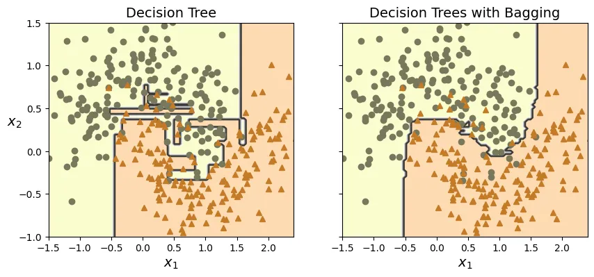
Đánh giá OOB (Out-of-Bag Evaluation)
Trong Bagging, với mỗi bộ phân loại, một số mẫu dữ liệu có thể được chọn nhiều lần, trong khi một số khác không được chọn lần nào. Những mẫu không được chọn gọi là Out-of-Bag (OOB).
Cơ sở Toán học: Nếu bạn lấy ngẫu nhiên một mẫu từ tập dữ liệu kích thước (có hoàn lại), xác suất để một mẫu cụ thể không được chọn là . Nếu lặp lại lần, xác suất để mẫu đó không bao giờ được chọn là . Khi , giới hạn này là: Nghĩa là khoảng 37% số mẫu sẽ không được sử dụng để huấn luyện (OOB), và 63% sẽ được sử dụng. Chúng ta có thể dùng 37% này làm tập kiểm tra (validation set) tự nhiên.
# Bật tính năng oob_score=True
bag_clf = BaggingClassifier(DecisionTreeClassifier(), n_estimators=500,
                            oob_score=True, n_jobs=-1, random_state=42)
bag_clf.fit(X_train, y_train)

# Xem điểm số OOB
bag_clf.oob_score_
output:
0.896Chúng ta cũng có thể xem xác suất dự đoán của các mẫu OOB:
bag_clf.oob_decision_function_[:3] # Xác suất cho 3 mẫu đầu tiênoutput:
array([[0.32352941, 0.67647059],
[0.3375 , 0.6625 ],
[1. , 0. ]])So sánh điểm OOB với độ chính xác thực tế trên tập kiểm tra:
from sklearn.metrics import accuracy_score
y_pred = bag_clf.predict(X_test)
accuracy_score(y_test, y_pred)
output:
0.92# extra code – tính toán xác suất 63%
print(1 - (1 - 1 / 1000) ** 1000)
print(1 - np.exp(-1))output:
0.6323045752290363
0.63212055882855773. Rừng ngẫu nhiên (Random Forests)
Rừng ngẫu nhiên (Random Forest) về cơ bản là một tập hợp các Cây quyết định, thường được huấn luyện bằng phương pháp Bagging. Tuy nhiên, nó thêm một lớp ngẫu nhiên nữa: khi tách một nút trong cây, thay vì tìm đặc trưng tốt nhất trong tất cả các đặc trưng, nó chỉ tìm trong một tập con ngẫu nhiên các đặc trưng. Điều này làm tăng tính đa dạng của các cây và giúp giảm overfitting (giảm phương sai).
from sklearn.ensemble import RandomForestClassifier

# Khởi tạo Random Forest với 500 cây
rnd_clf = RandomForestClassifier(n_estimators=500, max_leaf_nodes=16,
                                 n_jobs=-1, random_state=42)
rnd_clf.fit(X_train, y_train)
y_pred_rf = rnd_clf.predict(X_test)
Để chứng minh rằng Random Forest thực chất là Bagging của các Decision Tree với các tham số cụ thể, chúng ta có thể cấu hình BaggingClassifier để hoạt động giống hệt RandomForestClassifier. splitter="random" trong Decision Tree có nghĩa là chọn ngưỡng ngẫu nhiên, nhưng ở đây chúng ta dùng max_features để mô phỏng việc chọn tập con đặc trưng. (Lưu ý: đoạn code so sánh dưới đây mang tính minh họa ý tưởng, RandomForestClassifier tối ưu hơn).
# Một BaggingClassifier tương đương với RandomForest
bag_clf = BaggingClassifier(
    DecisionTreeClassifier(max_features="sqrt", max_leaf_nodes=16),
    n_estimators=500, n_jobs=-1, random_state=42)

# extra code – kiểm chứng dự đoán giống nhau
bag_clf.fit(X_train, y_train)
y_pred_bag = bag_clf.predict(X_test)
np.all(y_pred_bag == y_pred_rf)  # Kiểm tra xem kết quả có giống hệt nhau không
output:
np.True_Tầm quan trọng của đặc trưng (Feature Importance)
Một tính năng tuyệt vời của Random Forest là khả năng đo lường tầm quan trọng của từng đặc trưng (feature). Scikit-Learn đo lường điều này bằng cách xem xét mức độ giảm tạp chất (impurity) trung bình mà mỗi đặc trưng đóng góp trên tất cả các cây trong rừng (weighted average).
Dưới đây là ví dụ trên bộ dữ liệu hoa Iris:
from sklearn.datasets import load_iris
iris = load_iris(as_frame=True)

rnd_clf = RandomForestClassifier(n_estimators=500, random_state=42)
rnd_clf.fit(iris.data, iris.target)

for score, name in zip(rnd_clf.feature_importances_, iris.data.columns):
    print(round(score, 2), name)
output:
0.11 sepal length (cm)
0.02 sepal width (cm)
0.44 petal length (cm)
0.42 petal width (cm)Chúng ta cũng có thể áp dụng kỹ thuật này trên bộ dữ liệu MNIST để xem phần nào của hình ảnh (pixel nào) quan trọng nhất để phân loại các chữ số.
# extra code – ô này tạo ra Hình 6–6: Bản đồ nhiệt (heatmap) tầm quan trọng của pixel trên MNIST
from sklearn.datasets import fetch_openml

X_mnist, y_mnist = fetch_openml('mnist_784', return_X_y=True, as_frame=False,
                                parser='auto')

rnd_clf = RandomForestClassifier(n_estimators=100, random_state=42)
rnd_clf.fit(X_mnist, y_mnist)

heatmap_image = rnd_clf.feature_importances_.reshape(28, 28)
plt.imshow(heatmap_image, cmap="hot")
cbar = plt.colorbar(ticks=[rnd_clf.feature_importances_.min(),
                           rnd_clf.feature_importances_.max()])
cbar.ax.set_yticklabels(['Not important', 'Very important'], fontsize=14)
plt.axis("off")
plt.show()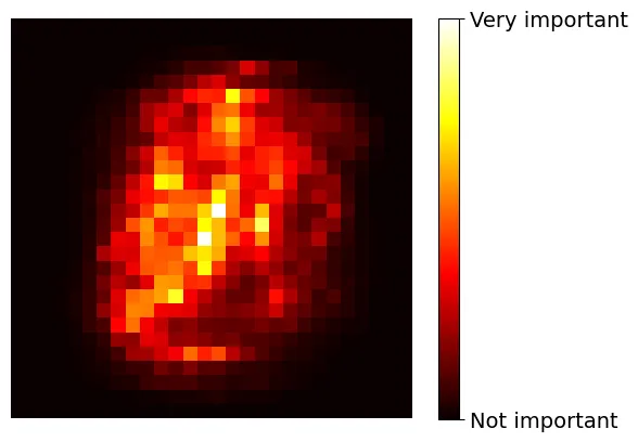
4. Boosting (Tăng cường)
Boosting là một kỹ thuật học kết hợp kết nối nhiều bộ phân loại yếu thành một bộ phân loại mạnh bằng cách huấn luyện các mô hình một cách tuần tự (sequential), trong đó mỗi mô hình cố gắng sửa chữa sai sót của mô hình trước đó.
AdaBoost (Adaptive Boosting)
Trong AdaBoost, mô hình mới sẽ tập trung nhiều hơn vào các mẫu dữ liệu mà mô hình trước đó đã phân loại sai.
Thuật toán:
- Khởi tạo trọng số mẫu .
- Huấn luyện bộ phân loại yếu. Tính tỷ lệ lỗi có trọng số :
- Tính trọng số bộ phân loại dựa trên learning rate :
- Cập nhật trọng số mẫu (tăng trọng số cho mẫu sai):
- Chuẩn hóa lại trọng số mẫu và lặp lại.
Đoạn mã dưới đây minh họa quá trình cập nhật trọng số và ranh giới quyết định của SVM qua 5 lần lặp.
# extra code – ô này tạo ra Hình 6–8 minh họa AdaBoost
m = len(X_train)  # số lượng mẫu

fig, axes = plt.subplots(ncols=2, figsize=(10, 4), sharey=True)
for subplot, learning_rate in ((0, 1), (1, 0.5)):
    sample_weights = np.ones(m) / m
    plt.sca(axes[subplot])
    for i in range(5):
        svm_clf = SVC(C=0.2, gamma=0.6, random_state=42)
        svm_clf.fit(X_train, y_train, sample_weight=sample_weights * m)
        y_pred = svm_clf.predict(X_train)

        error_weights = sample_weights[y_pred != y_train].sum()
        r = error_weights / sample_weights.sum()  # phương trình 7-1
        alpha = learning_rate * np.log((1 - r) / r)  # phương trình 7-2
        sample_weights[y_pred != y_train] *= np.exp(alpha)  # phương trình 7-3
        sample_weights /= sample_weights.sum()  # bước chuẩn hóa

        plot_decision_boundary(svm_clf, X_train, y_train, alpha=0.4)
        plt.title(f"learning_rate = {learning_rate}")
    if subplot == 0:
        plt.text(-0.75, -0.95, "1", fontsize=16)
        plt.text(-1.05, -0.95, "2", fontsize=16)
        plt.text(1.0, -0.95, "3", fontsize=16)
        plt.text(-1.45, -0.5, "4", fontsize=16)
        plt.text(1.36,  -0.95, "5", fontsize=16)
    else:
        plt.ylabel("")
plt.show()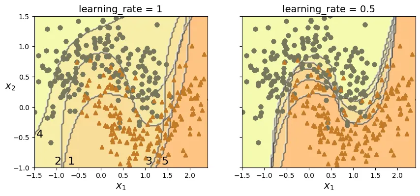
Sử dụng AdaBoostClassifier trong Scikit-Learn với mô hình cơ sở là Decision Stump (cây quyết định độ sâu 1).
from sklearn.ensemble import AdaBoostClassifier

# Khởi tạo AdaBoost với 30 cây quyết định độ sâu 1
ada_clf = AdaBoostClassifier(
    DecisionTreeClassifier(max_depth=1), n_estimators=30,
    learning_rate=0.5, random_state=42, algorithm="SAMME")
ada_clf.fit(X_train, y_train)
output:
AdaBoostClassifier(algorithm='SAMME',
estimator=DecisionTreeClassifier(max_depth=1),
learning_rate=0.5, n_estimators=30, random_state=42)# extra code – vẽ ranh giới quyết định của AdaBoost
plot_decision_boundary(ada_clf, X_train, y_train)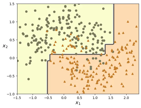
Gradient Boosting
Gradient Boosting cũng hoạt động tuần tự. Nhưng thay vì thay đổi trọng số của các mẫu dữ liệu như AdaBoost, phương pháp này cố gắng huấn luyện mô hình mới dựa trên sai số thặng dư (residual errors) của mô hình trước đó.
Giả sử mô hình hiện tại là , ta muốn tìm sao cho xấp xỉ . Điều này tương đương với việc huấn luyện để dự đoán (residuals).
Hãy cùng thực hiện Gradient Boosting thủ công với bài toán hồi quy (Regression).
import numpy as np
from sklearn.tree import DecisionTreeRegressor

# Tạo dữ liệu bậc 2 có nhiễu
m = 100
rng = np.random.default_rng(seed=42)
X = rng.random((m, 1)) - 0.5
noise = 0.05 * rng.standard_normal(m)
y = 3 * X[:, 0] ** 2 + noise  # y = 3x² + Gaussian noise

# Huấn luyện cây thứ nhất trên dữ liệu gốc
tree_reg1 = DecisionTreeRegressor(max_depth=2, random_state=42)
tree_reg1.fit(X, y)
output:
DecisionTreeRegressor(max_depth=2, random_state=42)Bây giờ, chúng ta tính toán sai số (residuals) của cây thứ nhất và huấn luyện cây thứ hai trên sai số này.
y2 = y - tree_reg1.predict(X)  # Tính sai số thặng dư
tree_reg2 = DecisionTreeRegressor(max_depth=2, random_state=43)
tree_reg2.fit(X, y2)  # Huấn luyện trên sai số
output:
DecisionTreeRegressor(max_depth=2, random_state=43)Tiếp tục làm tương tự với cây thứ ba.
y3 = y2 - tree_reg2.predict(X)
tree_reg3 = DecisionTreeRegressor(max_depth=2, random_state=44)
tree_reg3.fit(X, y3)
output:
DecisionTreeRegressor(max_depth=2, random_state=44)Dự đoán cuối cùng là tổng dự đoán của cả ba cây.
X_new = np.array([[-0.4], [0.], [0.5]])
sum(tree.predict(X_new) for tree in (tree_reg1, tree_reg2, tree_reg3))
output:
array([0.57356534, 0.0405142 , 0.66914249])Biểu đồ dưới đây minh họa quá trình này. Cột bên trái hiển thị dự đoán của từng cây riêng lẻ (trên residuals), cột bên phải hiển thị dự đoán tổng hợp của ensemble.
# extra code – ô này tạo ra Hình 6–9 minh họa Gradient Boosting
def plot_predictions(regressors, X, y, axes, style,
                     label=None, data_style="b.", data_label=None):
    x1 = np.linspace(axes[0], axes[1], 500)
    y_pred = sum(regressor.predict(x1.reshape(-1, 1))
                 for regressor in regressors)
    plt.plot(X[:, 0], y, data_style, label=data_label)
    plt.plot(x1, y_pred, style, linewidth=2, label=label)
    if label or data_label:
        plt.legend(loc="upper center")
    plt.axis(axes)

plt.figure(figsize=(11, 11))

plt.subplot(3, 2, 1)
plot_predictions([tree_reg1], X, y, axes=[-0.5, 0.5, -0.2, 0.8], style="g-",
                 label="$h_1(x_1)$", data_label="Training set")
plt.ylabel("$y$  ", rotation=0)
plt.title("Residuals and tree predictions")

plt.subplot(3, 2, 2)
plot_predictions([tree_reg1], X, y, axes=[-0.5, 0.5, -0.2, 0.8], style="r-",
                 label="$h(x_1) = h_1(x_1)$", data_label="Training set")
plt.title("Ensemble predictions")

plt.subplot(3, 2, 3)
plot_predictions([tree_reg2], X, y2, axes=[-0.5, 0.5, -0.4, 0.6], style="g-",
                 label="$h_2(x_1)$", data_style="k+",
                 data_label="Residuals: $y - h_1(x_1)$")
plt.ylabel("$y$  ", rotation=0)

plt.subplot(3, 2, 4)
plot_predictions([tree_reg1, tree_reg2], X, y, axes=[-0.5, 0.5, -0.2, 0.8],
                  style="r-", label="$h(x_1) = h_1(x_1) + h_2(x_1)$")

plt.subplot(3, 2, 5)
plot_predictions([tree_reg3], X, y3, axes=[-0.5, 0.5, -0.4, 0.6], style="g-",
                 label="$h_3(x_1)$", data_style="k+",
                 data_label="Residuals: $y - h_1(x_1) - h_2(x_1)$")
plt.xlabel("$x_1$")
plt.ylabel("$y$  ", rotation=0)

plt.subplot(3, 2, 6)
plot_predictions([tree_reg1, tree_reg2, tree_reg3], X, y,
                 axes=[-0.5, 0.5, -0.2, 0.8], style="r-",
                 label="$h(x_1) = h_1(x_1) + h_2(x_1) + h_3(x_1)$")
plt.xlabel("$x_1$")
plt.show()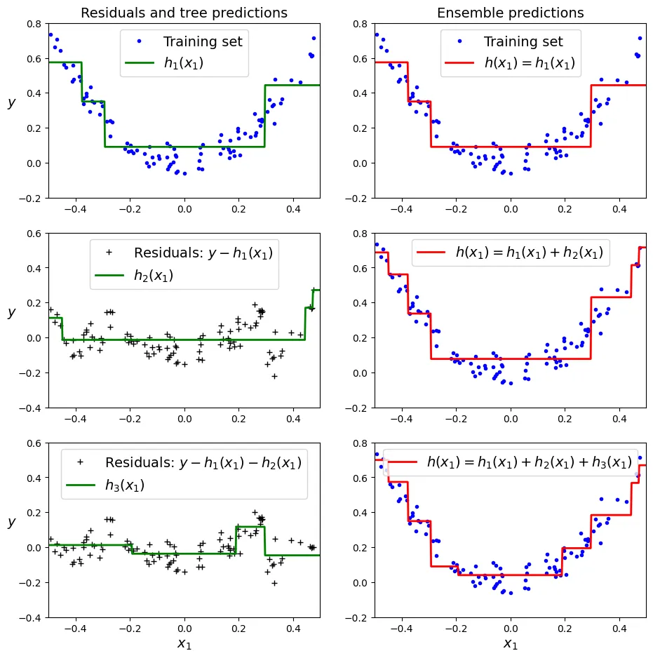
Scikit-Learn cung cấp lớp GradientBoostingRegressor. Tham số learning_rate kiểm soát mức độ đóng góp của mỗi cây. Tốc độ học thấp nghĩa là cần nhiều cây hơn, nhưng mô hình thường khái quát hóa tốt hơn (kỹ thuật Shrinkage).
from sklearn.ensemble import GradientBoostingRegressor

# Gradient Boosting cơ bản
gbrt = GradientBoostingRegressor(max_depth=2, n_estimators=3,
                                 learning_rate=1.0, random_state=42)
gbrt.fit(X, y)
output:
GradientBoostingRegressor(learning_rate=1.0, max_depth=2, n_estimators=3,
random_state=42)Để tìm số lượng cây tối ưu và tránh overfitting, chúng ta sử dụng kỹ thuật Dừng sớm (Early Stopping). Tham số n_iter_no_change sẽ dừng huấn luyện nếu validation score không cải thiện sau n vòng lặp.
# Gradient Boosting với Early Stopping
gbrt_best = GradientBoostingRegressor(
    max_depth=2, learning_rate=0.05, n_estimators=500,
    n_iter_no_change=10, random_state=42)
gbrt_best.fit(X, y)
output:
GradientBoostingRegressor(learning_rate=0.05, max_depth=2, n_estimators=500,
n_iter_no_change=10, random_state=42)# Số lượng cây thực tế được sử dụng
gbrt_best.n_estimators_output:
53Biểu đồ so sánh giữa việc chưa đủ cây (underfitting - bên trái) và số lượng cây tối ưu (bên phải).
# extra code – ô này tạo ra Hình 6–10
fig, axes = plt.subplots(ncols=2, figsize=(10, 4), sharey=True)

plt.sca(axes[0])
plot_predictions([gbrt], X, y, axes=[-0.5, 0.5, -0.1, 0.8], style="r-",
                 label="Ensemble predictions")
plt.title(f"learning_rate={gbrt.learning_rate}, "
          f"n_estimators={gbrt.n_estimators_}")
plt.xlabel("$x_1$")
plt.ylabel("$y$", rotation=0)

plt.sca(axes[1])
plot_predictions([gbrt_best], X, y, axes=[-0.5, 0.5, -0.1, 0.8], style="r-")
plt.title(f"learning_rate={gbrt_best.learning_rate}, "
          f"n_estimators={gbrt_best.n_estimators_}")
plt.xlabel("$x_1$")
plt.show()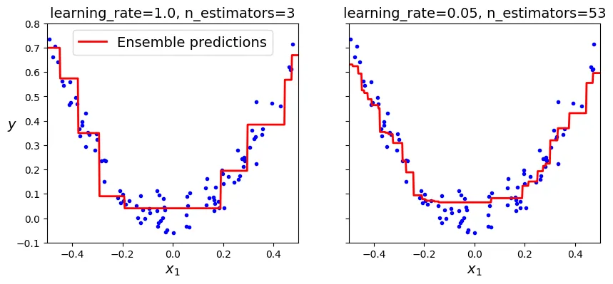
Histogram-based Gradient Boosting
Đối với các tập dữ liệu lớn, việc huấn luyện Gradient Boosting truyền thống rất chậm do phải tìm điểm chia (split point) trên tất cả các giá trị đặc trưng. Scikit-Learn cung cấp HistGradientBoostingRegressor. Nó chia các giá trị liên tục vào các bin (thùng) rời rạc (thường là 255 bin), giúp giảm độ phức tạp từ xuống .
Dưới đây, chúng ta sẽ tải dữ liệu nhà ở California để thử nghiệm.
# extra code – tải dữ liệu housing (tương tự chương 2)
from pathlib import Path
import tarfile
import urllib.request
import pandas as pd
from sklearn.model_selection import train_test_split

def load_housing_data():
    tarball_path = Path("datasets/housing.tgz")
    if not tarball_path.is_file():
        Path("datasets").mkdir(parents=True, exist_ok=True)
        url = "https://github.com/ageron/data/raw/main/housing.tgz"
        urllib.request.urlretrieve(url, tarball_path)
        with tarfile.open(tarball_path) as housing_tarball:
            housing_tarball.extractall(path="datasets")
    return pd.read_csv(Path("datasets/housing/housing.csv"))

housing = load_housing_data()
train_set, test_set = train_test_split(housing, test_size=0.2, random_state=42)
housing_labels = train_set["median_house_value"]
housing = train_set.drop("median_house_value", axis=1)
HistGradientBoostingRegressor cũng có khả năng xử lý trực tiếp các biến phân loại (categorical features) và các giá trị còn thiếu (missing values).
from sklearn.pipeline import make_pipeline
from sklearn.compose import make_column_transformer
from sklearn.ensemble import HistGradientBoostingRegressor
from sklearn.preprocessing import OrdinalEncoder

# Tạo pipeline xử lý dữ liệu và huấn luyện mô hình
hgb_reg = make_pipeline(
    make_column_transformer((OrdinalEncoder(), ["ocean_proximity"]),
                            remainder="passthrough",
                            force_int_remainder_cols=False),
    HistGradientBoostingRegressor(categorical_features=[0], random_state=42))

hgb_reg.fit(housing, housing_labels)
output:
Pipeline(steps=[('columntransformer',
ColumnTransformer(force_int_remainder_cols=False,
remainder='passthrough',
transformers=[('ordinalencoder',
OrdinalEncoder(),
['ocean_proximity'])])),
('histgradientboostingregressor',
HistGradientBoostingRegressor(categorical_features=[0],
random_state=42))])Đánh giá mô hình bằng RMSE thông qua cross-validation.
# extra code – đánh giá RMSE
from sklearn.model_selection import cross_val_score

hgb_rmses = -cross_val_score(hgb_reg, housing, housing_labels,
                             scoring="neg_root_mean_squared_error", cv=10)
pd.Series(hgb_rmses).describe()
output:
count 10.000000
mean 47613.307194
std 1295.422509
min 44963.213061
25% 47001.233485
50% 48000.963564
75% 48488.093243
max 49176.368465
dtype: float645. Stacking (Xếp chồng)
Stacking (Stacked Generalization) dựa trên ý tưởng đơn giản: thay vì dùng một hàm cố định (như biểu quyết cứng) để tổng hợp dự đoán, tại sao không huấn luyện một mô hình khác để thực hiện việc này? Mô hình tổng hợp này gọi là Blender hoặc Meta-learner.
Mô hình Blender nhận đầu vào là các dự đoán của các mô hình cơ sở (Base Estimators) và học cách kết hợp chúng để đưa ra dự đoán cuối cùng.
from sklearn.ensemble import StackingClassifier

# Khởi tạo StackingClassifier
stacking_clf = StackingClassifier(
    estimators=[
        ('lr', LogisticRegression(random_state=42)),
        ('rf', RandomForestClassifier(random_state=42)),
        ('svc', SVC(probability=True, random_state=42))
    ],
    final_estimator=RandomForestClassifier(random_state=43),
    cv=5  # số lượng fold cho cross-validation để huấn luyện blender
)
stacking_clf.fit(X_train, y_train)
output:
StackingClassifier(cv=5,
estimators=[('lr', LogisticRegression(random_state=42)),
('rf', RandomForestClassifier(random_state=42)),
('svc', SVC(probability=True, random_state=42))],
final_estimator=RandomForestClassifier(random_state=43))Đánh giá độ chính xác của mô hình Stacking.
stacking_clf.score(X_test, y_test)output:
0.928Ôn tập
- Sức mạnh của Ensemble: Nếu các mô hình cơ sở mắc các lỗi không tương quan nhau, việc kết hợp chúng sẽ triệt tiêu các lỗi ngẫu nhiên, giúp ensemble hoạt động tốt hơn mô hình đơn lẻ tốt nhất.
- Hard vs. Soft Voting: Soft voting (dựa trên xác suất) thường tốt hơn Hard voting (dựa trên đếm phiếu) vì nó coi trọng các dự đoán có độ tin cậy cao.
- Phân tán huấn luyện: Bagging/Pasting và Random Forest có thể huấn luyện song song dễ dàng. Boosting không thể huấn luyện song song vì tính chất tuần tự của nó. Stacking chỉ song song hóa được ở lớp (layer) đầu tiên.
- OOB: Giúp đánh giá mô hình Bagging “miễn phí” mà không cần tập validation riêng.
- Extra-Trees: Nhanh hơn Random Forest vì chọn ngưỡng ngẫu nhiên thay vì tìm tối ưu, dẫn đến bias cao hơn nhưng variance thấp hơn.
Bài tập thực hành 1: Voting Classifier trên MNIST
Bước 1: Chuẩn bị dữ liệu.
# Chia dữ liệu MNIST
X_train, y_train = X_mnist[:50_000], y_mnist[:50_000]
X_valid, y_valid = X_mnist[50_000:60_000], y_mnist[50_000:60_000]
X_test, y_test = X_mnist[60_000:], y_mnist[60_000:]
Bước 2: Huấn luyện các mô hình đơn lẻ.
from sklearn.ensemble import ExtraTreesClassifier
from sklearn.svm import LinearSVC
from sklearn.neural_network import MLPClassifier

random_forest_clf = RandomForestClassifier(n_estimators=100, random_state=42)
extra_trees_clf = ExtraTreesClassifier(n_estimators=100, random_state=42)
svm_clf = LinearSVC(max_iter=100, tol=20, dual=True, random_state=42)
mlp_clf = MLPClassifier(random_state=42)

estimators = [random_forest_clf, extra_trees_clf, svm_clf, mlp_clf]
for estimator in estimators:
    print("Training the", estimator)
    estimator.fit(X_train, y_train)
output:
Training the RandomForestClassifier(random_state=42)
Training the ExtraTreesClassifier(random_state=42)
Training the LinearSVC(dual=True, max_iter=100, random_state=42, tol=20)
Training the MLPClassifier(random_state=42)Bước 3: Đánh giá trên tập validation.
[estimator.score(X_valid, y_valid) for estimator in estimators]output:
[0.9736, 0.9743, 0.8662, 0.9613]Bước 4: Tạo VotingClassifier.
from sklearn.ensemble import VotingClassifier

named_estimators = [
    ("random_forest_clf", random_forest_clf),
    ("extra_trees_clf", extra_trees_clf),
    ("svm_clf", svm_clf),
    ("mlp_clf", mlp_clf),]

voting_clf = VotingClassifier(named_estimators)
voting_clf.fit(X_train, y_train)
voting_clf.score(X_valid, y_valid)
output:
0.975Bước 5: Tinh chỉnh Ensemble (Loại bỏ mô hình yếu). Cần chuyển đổi nhãn validation về dạng số để khớp với các estimator đã được clone bên trong VotingClassifier.
y_valid_encoded = y_valid.astype(np.int64)

# Loại bỏ SVM (hiệu năng thấp nhất)
voting_clf.set_params(svm_clf="drop")

# Cập nhật lại danh sách estimators
svm_clf_trained = voting_clf.named_estimators_.pop("svm_clf")
voting_clf.estimators_.remove(svm_clf_trained)

# Đánh giá lại
voting_clf.score(X_valid, y_valid)
output:
0.9761Thử nghiệm Soft Voting (Lưu ý: LinearSVC không hỗ trợ predict_proba nên phải bỏ qua hoặc dùng CalibratedClassifierCV, nhưng ở đây ta chỉ dùng các mô hình còn lại).
voting_clf.voting = "soft"
# (Ở đây cần đảm bảo tất cả mô hình còn lại hỗ trợ predict_proba)
# Random Forest, Extra Trees, MLP đều hỗ trợ.
print("Soft voting score:", voting_clf.score(X_valid, y_valid))
output:
Soft voting score: 0.9703Kết quả Hard Voting tốt hơn trong trường hợp này.
voting_clf.voting = "hard"
print("Hard voting score (test set):", voting_clf.score(X_test, y_test))
output:
Hard voting score (test set): 0.9733Bài tập thực hành 2: Stacking Ensemble
Bước 1: Tạo tập dữ liệu mới từ dự đoán của lớp 1 (Layer 1).
X_valid_predictions = np.empty((len(X_valid), len(estimators)), dtype=object)
for index, estimator in enumerate(estimators):
    X_valid_predictions[:, index] = estimator.predict(X_valid)
Bước 2: Huấn luyện Blender.
rnd_forest_blender = RandomForestClassifier(n_estimators=200, oob_score=True,
                                            random_state=42)
rnd_forest_blender.fit(X_valid_predictions, y_valid)
rnd_forest_blender.oob_score_
output:
0.9738Bước 3: Đánh giá trên tập kiểm tra.
X_test_predictions = np.empty((len(X_test), len(estimators)), dtype=object)
for index, estimator in enumerate(estimators):
    X_test_predictions[:, index] = estimator.predict(X_test)

y_pred = rnd_forest_blender.predict(X_test_predictions)
accuracy_score(y_test, y_pred)
output:
0.9688Bước 4: Sử dụng StackingClassifier của Scikit-Learn.
# Gộp tập train và valid lại vì StackingClassifier dùng CV nội bộ
X_train_full, y_train_full = X_mnist[:60_000], y_mnist[:60_000]

stack_clf = StackingClassifier(named_estimators,
                               final_estimator=rnd_forest_blender)
stack_clf.fit(X_train_full, y_train_full)
stack_clf.score(X_test, y_test)
output:
0.9795Kết quả StackingClassifier (0.9795) vượt trội hơn Voting Classifier và mọi mô hình đơn lẻ.