[ML101] Chương 5: Cây Quyết Định (Decision Trees)

Bài viết có tham khảo, sử dụng và sửa đổi tài nguyên từ kho lưu trữ handson-mlp, tuân thủ giấy phép Apache‑2.0. Chúng tôi chân thành cảm ơn tác giả Aurélien Géron (@aureliengeron) vì sự chia sẻ kiến thức tuyệt vời và những đóng góp quý giá cho cộng đồng.

Chương này sẽ hướng dẫn bạn tìm hiểu về Cây Quyết Định (Decision Trees), một thuật toán học máy phi tham số (non-parametric) linh hoạt và mạnh mẽ. Cây quyết định có khả năng thực hiện cả nhiệm vụ phân loại (classification) và hồi quy (regression), cũng như xử lý các bài toán có nhiều đầu ra (multioutput tasks). Đây là nền tảng cấu thành nên Rừng Ngẫu nhiên (Random Forests), một trong những thuật toán ensemble learning hiệu quả nhất hiện nay.

Chúng ta sẽ đi sâu vào cơ chế hoạt động của thuật toán CART (Classification and Regression Trees), cách tính toán độ đo tạp chất (impurity measures) như Gini hay Entropy, và các kỹ thuật tối ưu hóa mô hình thông qua điều chuẩn (regularization).

Bạn có thể chạy trực tiếp các đoạn mã code tại: Google Colab.

Thiết lập môi trường (Setup)

Trước tiên, chúng ta cần đảm bảo tính tương thích của môi trường thực thi.

import sys

# Kiểm tra phiên bản Python, yêu cầu >= 3.10
assert sys.version_info >= (3, 10)

Kiểm tra thư viện Scikit-Learn:

from packaging.version import Version
import sklearn

# Kiểm tra phiên bản Scikit-Learn, yêu cầu >= 1.6.1
assert Version(sklearn.__version__) >= Version("1.6.1")

Cấu hình thông số cho biểu đồ matplotlib:

import matplotlib.pyplot as plt

# Thiết lập kích thước phông chữ cho các thành phần biểu đồ
plt.rc('font', size=14)
plt.rc('axes', labelsize=14, titlesize=14)
plt.rc('legend', fontsize=14)
plt.rc('xtick', labelsize=10)
plt.rc('ytick', labelsize=10)

Huấn luyện và Trực quan hóa Cây Quyết Định

Để minh họa, chúng ta sử dụng bộ dữ liệu Iris. DecisionTreeClassifier trong Scikit-Learn thực hiện phân chia nhị phân (binary splitting) tại mỗi nút.

from sklearn.datasets import load_iris
from sklearn.tree import DecisionTreeClassifier

# Tải bộ dữ liệu Iris
iris = load_iris(as_frame=True)
# Lấy hai đặc trưng: chiều dài và chiều rộng cánh hoa
X_iris = iris.data[["petal length (cm)", "petal width (cm)"]].values
y_iris = iris.target

# Khởi tạo mô hình Cây Quyết Định với độ sâu tối đa là 2
tree_clf = DecisionTreeClassifier(max_depth=2, random_state=42)
# Huấn luyện mô hình với dữ liệu
tree_clf.fit(X_iris, y_iris)

output:
DecisionTreeClassifier(max_depth=2, random_state=42)

Trực quan hóa cây giúp ta hiểu rõ “luật” mà mô hình đã học được.

from sklearn.tree import export_graphviz

# Xuất mô hình cây ra file định dạng .dot
export_graphviz(
        tree_clf,
        out_file="my_iris_tree.dot",
        feature_names=["petal length (cm)", "petal width (cm)"],
        class_names=iris.target_names,
        rounded=True,
        filled=True
    )

from graphviz import Source
# Hiển thị cây từ file .dot
Source.from_file("my_iris_tree.dot")

# Mã bổ sung: Chuyển đổi file .dot sang .png bằng command line tool
!dot -Tpng "my_iris_tree.dot" -o "my_iris_tree.png"

Đưa ra Dự đoán (Making Predictions)

Cơ chế dự đoán của Cây quyết định dựa trên việc duyệt cây từ gốc đến lá. Tại mỗi nút, một kiểm định điều kiện (ví dụ: petal length <= 2.45) được thực hiện.

Độ đo Gini (Gini Impurity): Mỗi nút trong cây có một thuộc tính gini, đo lường mức độ “vẩn đục” (impurity) của nút đó. Một nút là “tinh khiết” (gini = 0) nếu tất cả các mẫu huấn luyện thuộc về cùng một lớp. Công thức Gini cho nút $i$: $G_i = 1 - \sum_{k=1}^{n} p_{i,k}^2$ Trong đó $p_{i,k}$ là tỷ lệ các mẫu thuộc lớp $k$ trong số các mẫu huấn luyện tại nút $i$.

Biểu đồ dưới đây minh họa các ranh giới quyết định (decision boundaries) được tạo ra bởi các ngưỡng (thresholds) trong cây.

import numpy as np
import matplotlib.pyplot as plt
from matplotlib.colors import ListedColormap

# Định nghĩa bảng màu tùy chỉnh
custom_cmap = ListedColormap(['#fafab0', '#9898ff', '#a0faa0'])

plt.figure(figsize=(8, 4))

# Tạo lưới điểm để vẽ ranh giới quyết định
lengths, widths = np.meshgrid(np.linspace(0, 7.2, 100), np.linspace(0, 3, 100))
X_iris_all = np.c_[lengths.ravel(), widths.ravel()]

# Dự đoán cho toàn bộ lưới điểm
y_pred = tree_clf.predict(X_iris_all).reshape(lengths.shape)

# Vẽ vùng quyết định
plt.contourf(lengths, widths, y_pred, alpha=0.3, cmap=custom_cmap)

# Vẽ các điểm dữ liệu thực tế
for idx, (name, style) in enumerate(zip(iris.target_names, ("yo", "bs", "g^"))):
    plt.plot(X_iris[:, 0][y_iris == idx], X_iris[:, 1][y_iris == idx],
             style, label=f"Iris {name}")

# Mã bổ sung: Làm đẹp biểu đồ (tương ứng Hình 5-2)
# Huấn luyện một cây sâu hơn để lấy các ngưỡng (chỉ dùng cho mục đích minh họa)
tree_clf_deeper = DecisionTreeClassifier(max_depth=3, random_state=42)
tree_clf_deeper.fit(X_iris, y_iris)
th0, th1, th2a, th2b = tree_clf_deeper.tree_.threshold[[0, 2, 3, 6]]

# Thiết lập nhãn trục
plt.xlabel("Petal length (cm)")
plt.ylabel("Petal width (cm)")

# Vẽ các đường ranh giới phân chia
plt.plot([th0, th0], [0, 3], "k-", linewidth=2)
plt.plot([th0, 7.2], [th1, th1], "k--", linewidth=2)
plt.plot([th2a, th2a], [0, th1], "k:", linewidth=2)
plt.plot([th2b, th2b], [th1, 3], "k:", linewidth=2)

# Thêm chú thích độ sâu (Depth)
plt.text(th0 - 0.05, 1.0, "Depth=0", horizontalalignment="right", fontsize=15)
plt.text(3.2, th1 + 0.02, "Depth=1", verticalalignment="bottom", fontsize=13)
plt.text(th2a + 0.05, 0.5, "(Depth=2)", fontsize=11)

plt.axis([0, 7.2, 0, 3])
plt.legend()
plt.show()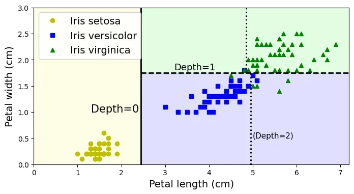

Cấu trúc cây được lưu trữ trong thuộc tính tree_:

# Truy cập đối tượng cấu trúc cây
tree_clf.tree_

output:
<sklearn.tree._tree.Tree at 0x79499dea5920>

# help(sklearn.tree._tree.Tree)

Ước lượng Xác suất Lớp (Estimating Class Probabilities)

Cây Quyết Định có thể trả về xác suất thuộc về từng lớp (class probability). Xác suất này chính là tỷ lệ các mẫu thuộc lớp đó trong nút lá tương ứng.

# Dự đoán xác suất cho mẫu [5, 1.5]
tree_clf.predict_proba([[5, 1.5]]).round(3)

output:
array([[0.   , 0.907, 0.093]])

# Dự đoán nhãn lớp cho mẫu [5, 1.5]
tree_clf.predict([[5, 1.5]])

output:
array([1])

Các Siêu tham số Điều chuẩn (Regularization Hyperparameters)

Cây Quyết Định là mô hình phi tham số, nghĩa là số lượng tham số không được xác định trước mà lớn lên theo dữ liệu. Điều này dẫn đến nguy cơ Overfitting (quá khớp) rất cao.

Để kiểm soát, chúng ta sử dụng các siêu tham số để giới hạn sự phát triển của cây:

• max_depth: Giới hạn độ sâu tối đa.
• min_samples_split: Số mẫu tối thiểu để một nút được phép phân chia.
• min_samples_leaf: Số mẫu tối thiểu phải có tại một nút lá.
• max_leaf_nodes: Số lượng nút lá tối đa.

Ví dụ minh họa sự khác biệt giữa mô hình không giới hạn (Overfitting) và mô hình có điều chuẩn trên bộ dữ liệu moons:

from sklearn.datasets import make_moons

# Tạo dữ liệu moons (dữ liệu hình trăng khuyết xen kẽ)
X_moons, y_moons = make_moons(n_samples=150, noise=0.2, random_state=42)

# Cây 1: Không có ràng buộc (mặc định)
tree_clf1 = DecisionTreeClassifier(random_state=42)

# Cây 2: Có ràng buộc min_samples_leaf=5
tree_clf2 = DecisionTreeClassifier(min_samples_leaf=5, random_state=42)

# Huấn luyện cả hai cây
tree_clf1.fit(X_moons, y_moons)
tree_clf2.fit(X_moons, y_moons)

output:
DecisionTreeClassifier(min_samples_leaf=5, random_state=42)

# Hàm hỗ trợ vẽ ranh giới quyết định
def plot_decision_boundary(clf, X, y, axes, cmap):
    x1, x2 = np.meshgrid(np.linspace(axes[0], axes[1], 100),
                         np.linspace(axes[2], axes[3], 100))
    X_new = np.c_[x1.ravel(), x2.ravel()]
    y_pred = clf.predict(X_new).reshape(x1.shape)

    plt.contourf(x1, x2, y_pred, alpha=0.3, cmap=cmap)
    plt.contour(x1, x2, y_pred, cmap="Greys", alpha=0.8)
    colors = {"Wistia": ["#78785c", "#c47b27"], "Pastel1": ["red", "blue"]}
    markers = ("o", "^")
    for idx in (0, 1):
        plt.plot(X[:, 0][y == idx], X[:, 1][y == idx],
                 color=colors[cmap][idx], marker=markers[idx], linestyle="none")
    plt.axis(axes)
    plt.xlabel(r"$x_1$")
    plt.ylabel(r"$x_2$", rotation=0)

fig, axes = plt.subplots(ncols=2, figsize=(10, 4), sharey=True)

# Vẽ cây không giới hạn
plt.sca(axes[0])
plot_decision_boundary(tree_clf1, X_moons, y_moons,
                       axes=[-1.5, 2.4, -1, 1.5], cmap="Wistia")
plt.title("No restrictions")

# Vẽ cây có giới hạn min_samples_leaf
plt.sca(axes[1])
plot_decision_boundary(tree_clf2, X_moons, y_moons,
                       axes=[-1.5, 2.4, -1, 1.5], cmap="Wistia")
plt.title(f"min_samples_leaf = {tree_clf2.min_samples_leaf}")
plt.ylabel("")
plt.show()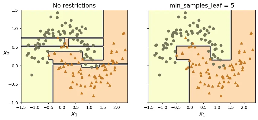

Đánh giá trên tập dữ liệu kiểm tra độc lập (test set) cho thấy mô hình có điều chuẩn hoạt động tốt hơn:

# Tạo tập test lớn hơn để đánh giá
X_moons_test, y_moons_test = make_moons(n_samples=1000, noise=0.2,
                                        random_state=43)

# Điểm số của cây không giới hạn
print(tree_clf1.score(X_moons_test, y_moons_test))

# Điểm số của cây có điều chuẩn
print(tree_clf2.score(X_moons_test, y_moons_test))

output:
0.898
0.92

Hồi quy (Regression)

Cây quyết định hồi quy hoạt động tương tự, nhưng thay vì dự đoán lớp, nó dự đoán một giá trị liên tục. Giá trị dự đoán của một nút lá là giá trị trung bình của các mẫu huấn luyện trong nút đó.

Hàm mất mát (Cost Function) cho hồi quy thường là MSE: $J(k, t_k) = \frac{m_{left}}{m} MSE_{left} + \frac{m_{right}}{m} MSE_{right}$ Trong đó thuật toán CART cố gắng phân chia để giảm thiểu MSE tổng hợp.

import numpy as np
from sklearn.tree import DecisionTreeRegressor

# Tạo dữ liệu bậc 2 ngẫu nhiên
rng = np.random.default_rng(seed=42)
X_quad = rng.random((200, 1)) - 0.5  # Một đặc trưng đầu vào ngẫu nhiên
y_quad = X_quad ** 2 + 0.025 * rng.standard_normal((200, 1)) # y = x^2 + nhiễu

# Huấn luyện cây hồi quy với độ sâu 2
tree_reg = DecisionTreeRegressor(max_depth=2, random_state=42)
tree_reg.fit(X_quad, y_quad)

output:
DecisionTreeRegressor(max_depth=2, random_state=42)

# Xuất cây hồi quy ra file .dot
export_graphviz(
    tree_reg,
    out_file="my_regression_tree.dot",
    feature_names=["x1"],
    rounded=True,
    filled=True)

# Hiển thị cây
Source.from_file("my_regression_tree.dot")

tree_reg2 = DecisionTreeRegressor(max_depth=3, random_state=42)
tree_reg2.fit(X_quad, y_quad)

output:
DecisionTreeRegressor(max_depth=3, random_state=42)

# Ngưỡng của cây độ sâu 2
tree_reg.tree_.threshold

output:
array([ 0.34304063, -0.30182856, -2.        , -2.        ,  0.43140428,
       -2.        , -2.        ])

# Ngưỡng của cây độ sâu 3
tree_reg2.tree_.threshold

output:
array([ 0.34304063, -0.30182856, -0.41395289, -2.        , -2.        ,
        0.21817657, -2.        , -2.        ,  0.43140428,  0.39480372,
       -2.        , -2.        ,  0.46470371, -2.        , -2.        ])

Biểu đồ so sánh độ sâu của cây hồi quy:

# Hàm vẽ dự đoán của cây hồi quy
def plot_regression_predictions(tree_reg, X, y, axes=[-0.5, 0.5, -0.05, 0.25]):
    x1 = np.linspace(axes[0], axes[1], 500).reshape(-1, 1)
    y_pred = tree_reg.predict(x1)
    plt.axis(axes)
    plt.xlabel("$x_1$")
    plt.plot(X, y, "b.")
    plt.plot(x1, y_pred, "r.-", linewidth=2, label=r"$\hat{y}$")

fig, axes = plt.subplots(ncols=2, figsize=(10, 4), sharey=True)

# Biểu đồ cho cây depth=2
plt.sca(axes[0])
plot_regression_predictions(tree_reg, X_quad, y_quad)
th0, th1a, th1b = tree_reg.tree_.threshold[[0, 1, 4]]
for split, style in ((th0, "k-"), (th1a, "k--"), (th1b, "k--")):
    plt.plot([split, split], [-0.05, 0.25], style, linewidth=2)
plt.text(th0, 0.16, "Depth=0", fontsize=15)
plt.text(th1a + 0.01, -0.01, "Depth=1", horizontalalignment="center", fontsize=13)
plt.text(th1b + 0.01, -0.01, "Depth=1", fontsize=13)
plt.ylabel("$y$", rotation=0)
plt.legend(loc="upper center", fontsize=16)
plt.title("max_depth=2")

# Biểu đồ cho cây depth=3
plt.sca(axes[1])
th2s = tree_reg2.tree_.threshold[[2, 5, 9, 12]]
plot_regression_predictions(tree_reg2, X_quad, y_quad)
for split, style in ((th0, "k-"), (th1a, "k--"), (th1b, "k--")):
    plt.plot([split, split], [-0.05, 0.25], style, linewidth=2)
for split in th2s:
    plt.plot([split, split], [-0.05, 0.25], "k:", linewidth=1)
plt.text(th2s[2] + 0.01, 0.15, "Depth=2", fontsize=13)
plt.title("max_depth=3")
plt.show()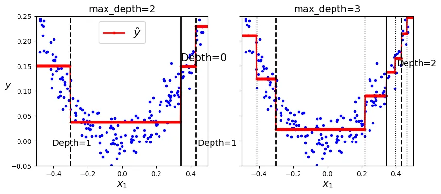

Cây hồi quy cũng dễ bị Overfitting nếu không được điều chuẩn:

# Tạo 2 cây hồi quy để so sánh điều chuẩn
tree_reg1 = DecisionTreeRegressor(random_state=42)
tree_reg2 = DecisionTreeRegressor(random_state=42, min_samples_leaf=10)

tree_reg1.fit(X_quad, y_quad)
tree_reg2.fit(X_quad, y_quad)

x1 = np.linspace(-0.5, 0.5, 500).reshape(-1, 1)
y_pred1 = tree_reg1.predict(x1)
y_pred2 = tree_reg2.predict(x1)

fig, axes = plt.subplots(ncols=2, figsize=(10, 4), sharey=True)

# Cây không giới hạn: Quá khớp nghiêm trọng
plt.sca(axes[0])
plt.plot(X_quad, y_quad, "b.")
plt.plot(x1, y_pred1, "r.-", linewidth=2, label=r"$\hat{y}$")
plt.axis([-0.5, 0.5, -0.05, 0.25])
plt.xlabel("$x_1$")
plt.ylabel("$y$", rotation=0)
plt.legend(loc="upper center")
plt.title("No restrictions")

# Cây có điều chuẩn: Mượt mà hơn
plt.sca(axes[1])
plt.plot(X_quad, y_quad, "b.")
plt.plot(x1, y_pred2, "r.-", linewidth=2, label=r"$\hat{y}$")
plt.axis([-0.5, 0.5, -0.05, 0.25])
plt.xlabel("$x_1$")
plt.title(f"min_samples_leaf={tree_reg2.min_samples_leaf}")
plt.show()

Độ nhạy cảm với hướng trục (Sensitivity to Axis Orientation)

Cây quyết định chia không gian dữ liệu bằng các đường thẳng vuông góc với trục tọa độ (orthogonal). Do đó, chúng rất nhạy cảm với việc xoay dữ liệu.

# Tạo dữ liệu hình vuông ngẫu nhiên
rng = np.random.default_rng(seed=42)
X_square = rng.random((100, 2)) - 0.5
y_square = (X_square[:, 0] > 0).astype(np.int64)

# Xoay dữ liệu 45 độ
angle = np.pi / 4  # 45 degrees
rotation_matrix = np.array([[np.cos(angle), -np.sin(angle)],
                            [np.sin(angle), np.cos(angle)]])
X_rotated_square = X_square.dot(rotation_matrix)

# Huấn luyện trên dữ liệu gốc
tree_clf_square = DecisionTreeClassifier(random_state=42)
tree_clf_square.fit(X_square, y_square)

# Huấn luyện trên dữ liệu đã xoay
tree_clf_rotated_square = DecisionTreeClassifier(random_state=42)
tree_clf_rotated_square.fit(X_rotated_square, y_square)

fig, axes = plt.subplots(ncols=2, figsize=(10, 4), sharey=True)

# Vẽ ranh giới dữ liệu gốc
plt.sca(axes[0])
plot_decision_boundary(tree_clf_square, X_square, y_square,
                       axes=[-0.7, 0.7, -0.7, 0.7], cmap="Pastel1")

# Vẽ ranh giới dữ liệu xoay
plt.sca(axes[1])
plot_decision_boundary(tree_clf_rotated_square, X_rotated_square, y_square,
                       axes=[-0.7, 0.7, -0.7, 0.7], cmap="Pastel1")
plt.ylabel("")
plt.show()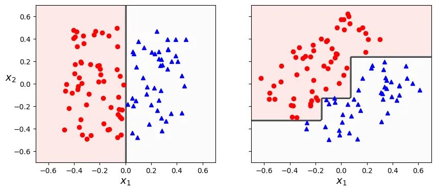

Giải pháp: Sử dụng PCA (Principal Component Analysis) để xoay dữ liệu sao cho các đặc trưng trở nên không tương quan (uncorrelated), giúp cây dễ dàng tìm ra ranh giới phân chia hơn.

from sklearn.decomposition import PCA
from sklearn.pipeline import make_pipeline
from sklearn.preprocessing import StandardScaler

# Tạo pipeline: Chuẩn hóa -> PCA -> Cây quyết định
pca_pipeline = make_pipeline(StandardScaler(), PCA())
X_iris_rotated = pca_pipeline.fit_transform(X_iris)
tree_clf_pca = DecisionTreeClassifier(max_depth=2, random_state=42)
tree_clf_pca.fit(X_iris_rotated, y_iris)

output:
DecisionTreeClassifier(max_depth=2, random_state=42)

plt.figure(figsize=(8, 4))
axes = [-2.2, 2.4, -0.6, 0.7]

# Tạo lưới điểm trên không gian đã biến đổi PCA
z0s, z1s = np.meshgrid(np.linspace(axes[0], axes[1], 100),
                       np.linspace(axes[2], axes[3], 100))
X_iris_pca_all = np.c_[z0s.ravel(), z1s.ravel()]
y_pred = tree_clf_pca.predict(X_iris_pca_all).reshape(z0s.shape)

plt.contourf(z0s, z1s, y_pred, alpha=0.3, cmap=custom_cmap)

# Vẽ dữ liệu đã xoay
for idx, (name, style) in enumerate(zip(iris.target_names, ("yo", "bs", "g^"))):
    plt.plot(X_iris_rotated[:, 0][y_iris == idx],
             X_iris_rotated[:, 1][y_iris == idx],
             style, label=f"Iris {name}")

plt.xlabel("$z_1$")
plt.ylabel("$z_2$", rotation=0)

# Vẽ đường phân chia của cây
th1, th2 = tree_clf_pca.tree_.threshold[[0, 2]]
plt.plot([th1, th1], axes[2:], "k-", linewidth=2)
plt.plot([th2, th2], axes[2:], "k--", linewidth=2)
plt.text(th1 - 0.01, axes[2] + 0.05, "Depth=0",
         horizontalalignment="right", fontsize=15)
plt.text(th2 - 0.01, axes[2] + 0.05, "Depth=1",
         horizontalalignment="right", fontsize=13)

plt.axis(axes)
plt.legend(loc=(0.32, 0.67))
plt.show()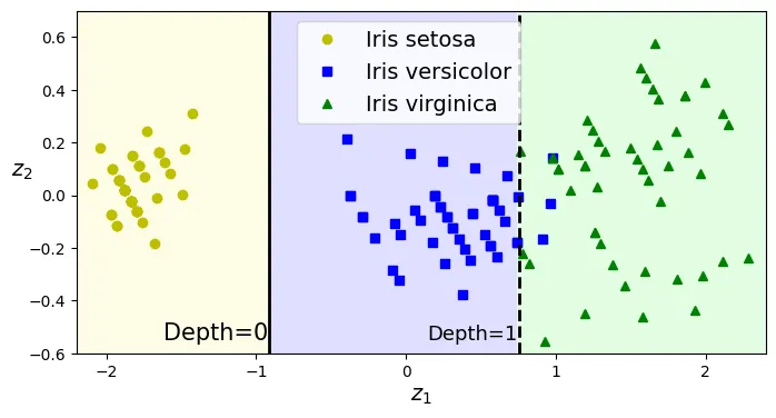

Cây Quyết Định có Phương sai Cao (High Variance)

Thuật toán huấn luyện cây là ngẫu nhiên (stochastic), nên ngay cả trên cùng một dữ liệu, các mô hình cũng có thể khác nhau nếu random_state thay đổi.

# Huấn luyện lại với random_state khác
tree_clf_tweaked = DecisionTreeClassifier(max_depth=2, random_state=40)
tree_clf_tweaked.fit(X_iris, y_iris)

output:
DecisionTreeClassifier(max_depth=2, random_state=40)

# Vẽ lại cây với random_state mới để thấy sự khác biệt (Hình 5-9)
plt.figure(figsize=(8, 4))
y_pred = tree_clf_tweaked.predict(X_iris_all).reshape(lengths.shape)
plt.contourf(lengths, widths, y_pred, alpha=0.3, cmap=custom_cmap)

for idx, (name, style) in enumerate(zip(iris.target_names, ("yo", "bs", "g^"))):
    plt.plot(X_iris[:, 0][y_iris == idx], X_iris[:, 1][y_iris == idx],
             style, label=f"Iris {name}")

th0, th1 = tree_clf_tweaked.tree_.threshold[[0, 2]]
plt.plot([0, 7.2], [th0, th0], "k-", linewidth=2)
plt.plot([0, 7.2], [th1, th1], "k--", linewidth=2)

plt.text(1.8, th0 + 0.05, "Depth=0", verticalalignment="bottom", fontsize=15)
plt.text(2.3, th1 + 0.05, "Depth=1", verticalalignment="bottom", fontsize=13)

plt.xlabel("Petal length (cm)")
plt.ylabel("Petal width (cm)")
plt.axis([0, 7.2, 0, 3])
plt.legend()
plt.show()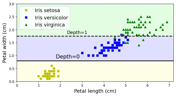

Tài liệu bổ sung: Cấu trúc cây (tree structure)

Phần này phân tích sâu vào đối tượng tree_ của Scikit-Learn.

tree = tree_clf.tree_
tree

output:
<sklearn.tree._tree.Tree at 0x79499dea5920>

tree.node_count

output:
5

tree.max_depth

output:
2

tree.max_n_classes

output:
3

tree.n_features

output:
2

tree.n_outputs

output:
1

tree.n_leaves

output:
np.int64(3)

tree.impurity

output:
array([0.66666667, 0.        , 0.5       , 0.16803841, 0.04253308])

tree.children_left[0], tree.children_right[0]

output:
(np.int64(1), np.int64(2))

tree.children_left[3], tree.children_right[3]

output:
(np.int64(-1), np.int64(-1))

is_leaf = (tree.children_left == tree.children_right)
np.arange(tree.node_count)[is_leaf]

output:
array([1, 3, 4])

tree.feature

output:
array([ 0, -2,  1, -2, -2], dtype=int64)

tree.threshold

output:
array([ 2.44999999, -2.        ,  1.75      , -2.        , -2.        ])

tree.value

output:
array([[[0.33333333, 0.33333333, 0.33333333]],

       [[1.        , 0.        , 0.        ]],

       [[0.        , 0.5       , 0.5       ]],

       [[0.        , 0.90740741, 0.09259259]],

       [[0.        , 0.02173913, 0.97826087]]])

tree.n_node_samples

output:
array([150,  50, 100,  54,  46], dtype=int64)

# Kiểm tra tính nhất quán: tổng samples theo class phải bằng n_node_samples
np.all(tree.value.sum(axis=(1, 2)) == tree.n_node_samples)

output:
np.False_

def compute_depth(tree_clf):
    tree = tree_clf.tree_
    depth = np.zeros(tree.node_count)
    stack = [(0, 0)]
    while stack:
        node, node_depth = stack.pop()
        depth[node] = node_depth
        if tree.children_left[node] != tree.children_right[node]:
            stack.append((tree.children_left[node], node_depth + 1))
            stack.append((tree.children_right[node], node_depth + 1))
    return depth

depth = compute_depth(tree_clf)
depth

output:
array([0., 1., 1., 2., 2.])

tree_clf.tree_.feature[(depth == 1) & (~is_leaf)]

output:
array([1], dtype=int64)

tree_clf.tree_.threshold[(depth == 1) & (~is_leaf)]

output:
array([1.75])

Ôn tập

Bài tập thực hành 1: Tinh chỉnh Hyperparameters cho dataset Moons

a. Tạo dữ liệu:

from sklearn.datasets import make_moons

# Tạo dữ liệu moons lớn
X_moons, y_moons = make_moons(n_samples=10000, noise=0.4, random_state=42)

b. Chia tập dữ liệu:

from sklearn.model_selection import train_test_split

X_train, X_test, y_train, y_test = train_test_split(X_moons, y_moons,
                                                    test_size=0.2,
                                                    random_state=42)

c. Tìm kiếm lưới (Grid Search):

from sklearn.model_selection import GridSearchCV

params = {
    'max_leaf_nodes': list(range(2, 100)),
    'max_depth': [1, 2, 3, 4, 5, 6],
    'min_samples_split': [2, 3, 4]}

grid_search_cv = GridSearchCV(DecisionTreeClassifier(random_state=42),
                              params,
                              cv=3)

grid_search_cv.fit(X_train, y_train)

output:
GridSearchCV(cv=3, estimator=DecisionTreeClassifier(random_state=42),
             param_grid={'max_depth': [1, 2, 3, 4, 5, 6],
                         'max_leaf_nodes': [2, 3, 4, 5, 6, 7, 8, 9, 10, 11, 12,
                                            13, 14, 15, 16, 17, 18, 19, 20, 21,
                                            22, 23, 24, 25, 26, 27, 28, 29, 30,
                                            31, ...],
                         'min_samples_split': [2, 3, 4]})

# Hiển thị bộ tham số tốt nhất tìm được
grid_search_cv.best_estimator_

output:
DecisionTreeClassifier(max_depth=6, max_leaf_nodes=17, random_state=42)

d. Đánh giá mô hình:

from sklearn.metrics import accuracy_score

y_pred = grid_search_cv.predict(X_test)
accuracy_score(y_test, y_pred)

output:
0.8595

Bài tập thực hành 2: Trồng một Rừng cây (Grow a Forest)

Xây dựng mô hình Random Forest từ đầu.

a. Tạo các tập con:

from sklearn.model_selection import ShuffleSplit

n_trees = 1000
n_instances = 100
mini_sets = []

# Sử dụng ShuffleSplit để lấy ngẫu nhiên các tập con
rs = ShuffleSplit(n_splits=n_trees, test_size=len(X_train) - n_instances,
                  random_state=42)

for mini_train_index, mini_test_index in rs.split(X_train):
    X_mini_train = X_train[mini_train_index]
    y_mini_train = y_train[mini_train_index]
    mini_sets.append((X_mini_train, y_mini_train))

b. Huấn luyện các cây:

from sklearn.base import clone

# Tạo danh sách 1000 cây (bản sao của mô hình tốt nhất)
forest = [clone(grid_search_cv.best_estimator_) for _ in range(n_trees)]
accuracy_scores = []

for tree, (X_mini_train, y_mini_train) in zip(forest, mini_sets):
    tree.fit(X_mini_train, y_mini_train)

    y_pred = tree.predict(X_test)
    accuracy_scores.append(accuracy_score(y_test, y_pred))

# Độ chính xác trung bình của các cây đơn lẻ (khoảng 80%)
np.mean(accuracy_scores)

output:
np.float64(0.8056605)

c. Tổng hợp dự đoán (Majority Vote):

Y_pred = np.empty([n_trees, len(X_test)], dtype=np.uint8)

# Thu thập dự đoán từ tất cả các cây
for tree_index, tree in enumerate(forest):
    Y_pred[tree_index] = tree.predict(X_test)

from scipy.stats import mode
# Tìm mode (giá trị xuất hiện nhiều nhất) cho mỗi mẫu
y_pred_majority_votes, n_votes = mode(Y_pred, axis=0)

d. Đánh giá kết quả cuối cùng:

accuracy_score(y_test, y_pred_majority_votes.reshape([-1]))

output:
0.873