[ML101] Chương 4: Huấn luyện Mô hình (Training Models)
Các phương pháp huấn luyện mô hình Machine Learning, gradient descent và regularization
Bài viết có tham khảo, sử dụng và sửa đổi tài nguyên từ kho lưu trữ handson-mlp, tuân thủ giấy phép Apache‑2.0. Chúng tôi chân thành cảm ơn tác giả Aurélien Géron (@aureliengeron) vì sự chia sẻ kiến thức tuyệt vời và những đóng góp quý giá cho cộng đồng.
Trong các chương trước, chúng ta đã sử dụng các mô hình Machine Learning như những “hộp đen” (black boxes): đưa dữ liệu vào và nhận kết quả đầu ra mà không thực sự đi sâu vào cơ chế hoạt động bên trong. Trong chương này, chúng ta sẽ mở những chiếc hộp đó ra để tìm hiểu nền tảng toán học, cách thức hoạt động, quy trình huấn luyện và các thuật toán tối ưu hóa tham số nội tại.
Việc hiểu rõ cơ chế hoạt động sẽ giúp bạn:
- Lựa chọn mô hình phù hợp cho bài toán cụ thể.
- Chọn thuật toán huấn luyện thích hợp (ví dụ: Batch GD so với SGD).
- Tinh chỉnh các siêu tham số (hyperparameters) hiệu quả hơn.
- Phân tích và khắc phục lỗi (debug) khi mô hình hoạt động không như ý muốn (ví dụ: underfitting hay overfitting).
Bạn có thể chạy trực tiếp các đoạn mã code tại: Google Colab.
Cài đặt và Khởi tạo (Setup)
Trước tiên, chúng ta cần đảm bảo môi trường Python và các thư viện cần thiết (như Scikit-Learn) đáp ứng yêu cầu phiên bản tối thiểu để đảm bảo tính tương thích.
# Dự án này yêu cầu Python 3.10 trở lên
import sys
assert sys.version_info >= (3, 10)
# Yêu cầu Scikit-Learn ≥ 1.6.1
from packaging.version import Version
import sklearn
assert Version(sklearn.__version__) >= Version("1.6.1")Chúng ta sẽ thiết lập kích thước phông chữ mặc định cho thư viện matplotlib để các biểu đồ hiển thị rõ ràng và thẩm mỹ hơn, hỗ trợ việc phân tích trực quan.
import matplotlib.pyplot as plt

# Thiết lập kích thước phông chữ cho các thành phần biểu đồ
plt.rc('font', size=14)
plt.rc('axes', labelsize=14, titlesize=14)
plt.rc('legend', fontsize=14)
plt.rc('xtick', labelsize=10)
plt.rc('ytick', labelsize=10)
Hồi quy Tuyến tính (Linear Regression)
Một mô hình hồi quy tuyến tính đưa ra dự đoán bằng cách tính tổng trọng số của các đặc trưng đầu vào cộng với một hằng số (được gọi là bias hay intercept).
Phương trình tổng quát dưới dạng vector:
Trong đó:
- là giá trị dự đoán.
- là vector đặc trưng của mẫu dữ liệu (với ).
- là vector tham số của mô hình (với là bias).
- là hàm giả thuyết (hypothesis function).
Để huấn luyện mô hình, ta cần tìm bộ tham số sao cho giảm thiểu sai số dự đoán trên tập huấn luyện. Thước đo phổ biến nhất cho bài toán hồi quy là Sai số Bình phương Trung bình (Mean Squared Error - MSE):
Phương trình Pháp tuyến (The Normal Equation)
Để tìm ra giá trị tối ưu nhằm cực tiểu hóa hàm mất mát MSE, tồn tại một giải pháp dạng đóng (closed-form solution) được gọi là Phương trình Pháp tuyến:
Hãy cùng tạo ra một bộ dữ liệu giả lập dạng tuyến tính để thử nghiệm tính đúng đắn của phương trình này.
import numpy as np

rng = np.random.default_rng(seed=42) # Khởi tạo bộ sinh số ngẫu nhiên
m = 200  # số lượng mẫu dữ liệu (instances)

# Tạo dữ liệu X ngẫu nhiên phân phối đều
X = 2 * rng.random((m, 1))  # vector cột

# Tạo dữ liệu y có mối quan hệ tuyến tính với X (y = 4 + 3x + nhiễu Gaussian)
y = 4 + 3 * X + rng.standard_normal((m, 1))  # vector cột
# đoạn code phụ – dùng để tạo Hình 4–1
import matplotlib.pyplot as plt
plt.figure(figsize=(6, 4))
plt.plot(X, y, "b.") # Vẽ các điểm dữ liệu màu xanh
plt.xlabel("$x_1$")
plt.ylabel("$y$", rotation=0)
plt.axis([0, 2, 0, 15]) # Giới hạn trục toạ độ
plt.grid()
plt.show()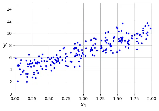
Bây giờ, chúng ta sẽ sử dụng Phương trình Pháp tuyến để tính toán . Chúng ta sẽ sử dụng hàm inv() từ mô-đun đại số tuyến tính của NumPy (np.linalg) để tính nghịch đảo ma trận, và toán tử @ để thực hiện nhân ma trận.
from sklearn.preprocessing import add_dummy_feature

# Thêm x0 = 1 vào mỗi mẫu dữ liệu (để nhân với theta_0 - bias term)
X_b = add_dummy_feature(X)

# Áp dụng công thức Phương trình Pháp tuyến: (X^T * X)^-1 * X^T * y
theta_best = np.linalg.inv(X_b.T @ X_b) @ X_b.T @ ytheta_bestoutput:
array([[3.69084138],
[3.32960458]])Chúng ta hy vọng và . Kết quả nhận được là và . Sự sai lệch này là do nhiễu Gaussian mà chúng ta đã thêm vào dữ liệu ().
Bây giờ ta có thể sử dụng để đưa ra dự đoán cho các giá trị mới bằng phép nhân ma trận:
X_new = np.array([[0], [2]])
X_new_b = add_dummy_feature(X_new)  # thêm x0 = 1 vào mỗi mẫu
y_predict = X_new_b @ theta_best
y_predict
output:
array([[ 3.69084138],
[10.35005055]])Hãy vẽ mô hình dự đoán (đường hồi quy) đè lên dữ liệu thực tế để kiểm chứng trực quan:
import matplotlib.pyplot as plt

plt.figure(figsize=(6, 4))  # đoạn code phụ – định dạng biểu đồ
plt.plot(X_new, y_predict, "r-", label="Predictions") # Vẽ đường dự đoán màu đỏ
plt.plot(X, y, "b.") # Vẽ dữ liệu thực tế

# đoạn code phụ – làm đẹp cho Hình 4–2
plt.xlabel("$x_1$")
plt.ylabel("$y$", rotation=0)
plt.axis([0, 2, 0, 15])
plt.grid()
plt.legend(loc="upper left")
plt.show()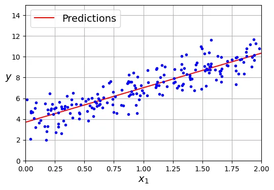
Thực hiện Hồi quy Tuyến tính bằng Scikit-Learn rất đơn giản với lớp LinearRegression. Lớp này đã tối ưu hóa việc tính toán.
from sklearn.linear_model import LinearRegression

lin_reg = LinearRegression()
lin_reg.fit(X, y)

# Hiển thị bias (intercept_) và trọng số (coef_)
lin_reg.intercept_, lin_reg.coef_
output:
(array([3.69084138]), array([[3.32960458]]))# Dự đoán giá trị mới
lin_reg.predict(X_new)output:
array([[ 3.69084138],
[10.35005055]])Lưu ý về thuật toán: Lớp LinearRegression thực chất dựa trên hàm scipy.linalg.lstsq() (Least Squares). Nó không tính toán trực tiếp vì độ phức tạp tính toán cao () và vấn đề ma trận không khả nghịch. Thay vào đó, nó sử dụng phân rã giá trị suy biến (Singular Value Decomposition - SVD) để tính ma trận giả nghịch đảo (pseudoinverse) .
Công thức: .
theta_best_svd, residuals, rank, s = np.linalg.lstsq(X_b, y, rcond=1e-6)
theta_best_svd
output:
array([[3.69084138],
[3.32960458]])Bạn có thể tính trực tiếp giả nghịch đảo bằng np.linalg.pinv():
np.linalg.pinv(X_b) @ youtput:
array([[3.69084138],
[3.32960458]])Gradient Descent (Hạ độ dốc)
Gradient Descent là một thuật toán tối ưu hóa tổng quát. Ý tưởng cốt lõi là tinh chỉnh các tham số lặp đi lặp lại để cực tiểu hóa hàm chi phí (cost function).
Hãy tưởng tượng bạn đang bị lạc trên núi trong sương mù dày đặc; bạn chỉ cảm nhận được độ dốc của mặt đất dưới chân. Chiến lược tốt nhất để xuống thung lũng nhanh chóng là đi theo hướng dốc xuống mạnh nhất. Gradient Descent hoạt động theo cách tương tự: nó đo gradient cục bộ của hàm lỗi theo vector tham số , và đi ngược hướng gradient đó. Khi gradient bằng 0, bạn đã đạt đến điểm cực tiểu (minimum).
Batch Gradient Descent (Hạ độ dốc toàn cục)
Để thực hiện Gradient Descent, bạn cần tính gradient của hàm chi phí đối với từng tham số mô hình . Vector gradient chứa tất cả các đạo hàm riêng này được ký hiệu là .
Công thức Gradient cho MSE:
Công thức cập nhật tham số (Gradient Descent Step):
Trong đó là tốc độ học (learning rate).
eta = 0.1  # learning rate (tốc độ học)
n_epochs = 1000 # số lần lặp lại quy trình huấn luyện
m = len(X_b)  # số lượng mẫu dữ liệu

rng = np.random.default_rng(seed=42)
theta = rng.standard_normal((2, 1))  # khởi tạo tham số ngẫu nhiên

for epoch in range(n_epochs):
    # Tính gradient của hàm loss MSE trên toàn bộ tập dữ liệu
    gradients = 2 / m * X_b.T @ (X_b @ theta - y)
    # Cập nhật theta
    theta = theta - eta * gradients
Sau khi huấn luyện, hãy xem các tham số mô hình thu được:
thetaoutput:
array([[3.69084138],
[3.32960458]])Kết quả này khớp chính xác với những gì Phương trình Pháp tuyến đã tìm ra. Gradient Descent đã hoạt động hoàn hảo.
Tuy nhiên, tốc độ học đóng vai trò rất quan trọng. Hình dưới đây sẽ minh họa quá trình Gradient Descent với ba giá trị tốc độ học khác nhau.
# đoạn code phụ – tạo Hình 4–8
import matplotlib as mpl

def plot_gradient_descent(theta, eta):
    m = len(X_b)
    plt.plot(X, y, "b.")
    n_epochs = 1000
    n_shown = 20
    theta_path = []
    for epoch in range(n_epochs):
        if epoch < n_shown:
            y_predict = X_new_b @ theta
            # Thay đổi màu sắc đường dự đoán dần dần từ nhạt sang đậm
            color = mpl.colors.rgb2hex(plt.cm.OrRd(epoch / n_shown + 0.15))
            plt.plot(X_new, y_predict, linestyle="solid", color=color)
        gradients = 2 / m * X_b.T @ (X_b @ theta - y)
        theta = theta - eta * gradients
        theta_path.append(theta)
    plt.xlabel("$x_1$")
    plt.axis([0, 2, 0, 15])
    plt.grid()
    plt.title(fr"$\eta = {eta}$")
    return theta_path

rng = np.random.default_rng(seed=42)
theta = rng.standard_normal((2, 1))  # khởi tạo tham số ngẫu nhiên

plt.figure(figsize=(10, 4))
plt.subplot(131)
plot_gradient_descent(theta, eta=0.02)
plt.ylabel("$y$", rotation=0)

plt.subplot(132)
theta_path_bgd = plot_gradient_descent(theta, eta=0.1)
plt.gca().axes.yaxis.set_ticklabels([])

plt.subplot(133)
plt.gca().axes.yaxis.set_ticklabels([])
plot_gradient_descent(theta, eta=0.5)
plt.show()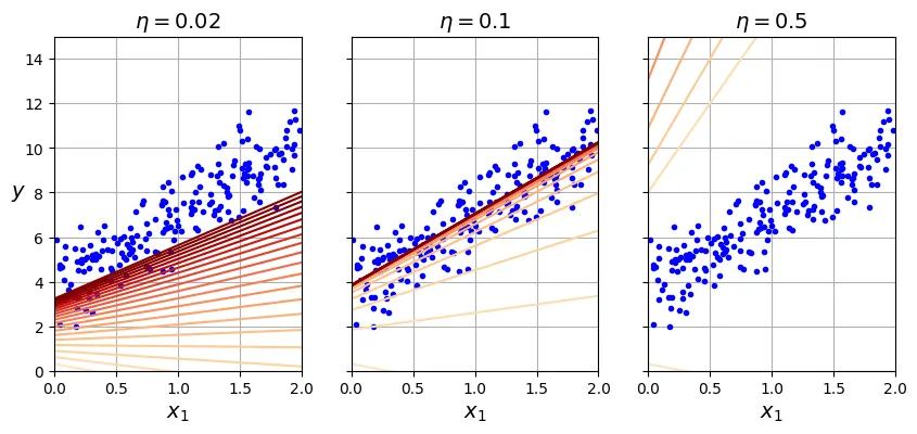
- Bên trái (): Quá thấp, thuật toán sẽ hội tụ nhưng mất rất nhiều thời gian.
- Ở giữa (): Vừa phải, hội tụ nhanh chóng sau vài bước lặp.
- Bên phải (): Quá cao, thuật toán nhảy vọt qua điểm cực tiểu và phân kỳ (diverge), ngày càng xa điểm tối ưu.
Stochastic Gradient Descent (Hạ độ dốc ngẫu nhiên)
Vấn đề chính của Batch Gradient Descent là nó sử dụng toàn bộ tập huấn luyện để tính gradient tại mỗi bước, khiến nó rất chậm khi lớn. Stochastic Gradient Descent (SGD) giải quyết vấn đề này bằng cách chọn ngẫu nhiên một mẫu dữ liệu tại mỗi bước và tính gradient chỉ dựa trên mẫu đó.
Do tính ngẫu nhiên, SGD ít ổn định hơn Batch GD. Hàm chi phí sẽ nảy lên xuống, giảm dần theo trung bình nhưng không bao giờ ổn định hoàn toàn tại một điểm. Để giúp thuật toán hội tụ, chúng ta cần giảm dần tốc độ học theo thời gian (learning schedule).
theta_path_sgd = []  # dùng để lưu đường đi của theta để vẽ biểu đồ sau này

n_epochs = 50
t0, t1 = 5, 50  # siêu tham số cho lịch trình học (learning schedule)

def learning_schedule(t):
    return t0 / (t + t1)

rng = np.random.default_rng(seed=42)
theta = rng.standard_normal((2, 1))  # khởi tạo tham số ngẫu nhiên

n_shown = 20  # chỉ vẽ 20 bước đầu tiên

plt.figure(figsize=(6, 4))  # đoạn code phụ – định dạng biểu đồ

for epoch in range(n_epochs):
    for iteration in range(m):

        # đoạn code phụ – vẽ các đường dự đoán trong quá trình học
        if epoch == 0 and iteration < n_shown:
            y_predict = X_new_b @ theta
            color = mpl.colors.rgb2hex(plt.cm.OrRd(iteration / n_shown + 0.15))
            plt.plot(X_new, y_predict, color=color)

        # Chọn ngẫu nhiên một mẫu dữ liệu
        random_index = rng.integers(m)
        xi = X_b[random_index : random_index + 1]
        yi = y[random_index : random_index + 1]

        # Tính gradient dựa trên mẫu đơn lẻ này
        gradients = 2 * xi.T @ (xi @ theta - yi)  # SGD không chia cho m

        # Cập nhật learning rate và theta
        eta = learning_schedule(epoch * m + iteration)
        theta = theta - eta * gradients
        theta_path_sgd.append(theta)  # lưu lại để vẽ sau

# đoạn code phụ – làm đẹp Hình 4–10
plt.plot(X, y, "b.")
plt.xlabel("$x_1$")
plt.ylabel("$y$", rotation=0)
plt.axis([0, 2, 0, 15])
plt.grid()
plt.show()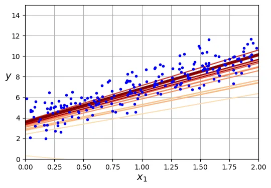
thetaoutput:
array([[3.69826475],
[3.30748311]])Trong Scikit-Learn, chúng ta có thể thực hiện SGD cho hồi quy tuyến tính bằng lớp SGDRegressor.
from sklearn.linear_model import SGDRegressor

# Chạy SGD tối đa 1000 epochs, dừng nếu loss không cải thiện quá 1e-5 (tol)
# penalty=None nghĩa là không dùng regularization (sẽ học sau)
sgd_reg = SGDRegressor(max_iter=1000, tol=1e-5, penalty=None, eta0=0.01,
                       n_iter_no_change=100, random_state=42)

sgd_reg.fit(X, y.ravel())  # y.ravel() vì fit() yêu cầu mảng 1 chiều cho target

sgd_reg.intercept_, sgd_reg.coef_
output:
(array([3.68899733]), array([3.33054574]))Mini-batch Gradient Descent
Mini-batch Gradient Descent là sự kết hợp giữa Batch GD và SGD. Thay vì tính gradient trên toàn bộ dữ liệu hay chỉ một mẫu, nó tính trên một tập hợp nhỏ ngẫu nhiên các mẫu gọi là mini-batch.
Ưu điểm chính của Mini-batch GD so với SGD là bạn có thể tận dụng khả năng tính toán ma trận song song của phần cứng (đặc biệt là GPU).
Đoạn mã dưới đây minh họa Mini-batch GD và so sánh đường đi của tham số trong không gian tham số giữa ba thuật toán.
# đoạn code phụ – tạo Hình 4–11
from math import ceil

n_epochs = 50
minibatch_size = 20
n_batches_per_epoch = ceil(m / minibatch_size)

rng = np.random.default_rng(seed=42)
theta = rng.standard_normal((2, 1))

t0, t1 = 200, 1000

def learning_schedule(t):
    return t0 / (t + t1)

theta_path_mgd = []

for epoch in range(n_epochs):
    # Xáo trộn dữ liệu đầu mỗi epoch để tránh lặp lại thứ tự
    shuffled_indices = rng.permutation(m)
    X_b_shuffled = X_b[shuffled_indices]
    y_shuffled = y[shuffled_indices]

    for iteration in range(0, n_batches_per_epoch):
        idx = iteration * minibatch_size
        xi = X_b_shuffled[idx : idx + minibatch_size]
        yi = y_shuffled[idx : idx + minibatch_size]

        gradients = 2 / minibatch_size * xi.T @ (xi @ theta - yi)
        eta = learning_schedule(epoch * n_batches_per_epoch + iteration)
        theta = theta - eta * gradients
        theta_path_mgd.append(theta)

theta_path_bgd = np.array(theta_path_bgd)
theta_path_sgd = np.array(theta_path_sgd)
theta_path_mgd = np.array(theta_path_mgd)

plt.figure(figsize=(7, 4))
plt.plot(theta_path_sgd[:, 0], theta_path_sgd[:, 1], "r-s", linewidth=1,
         label="Stochastic")
plt.plot(theta_path_mgd[:, 0], theta_path_mgd[:, 1], "g-+", linewidth=2,
         label="Mini-batch")
plt.plot(theta_path_bgd[:, 0], theta_path_bgd[:, 1], "b-o", linewidth=3,
         label="Batch")
plt.legend(loc="upper left")
plt.xlabel(r"$\theta_0$")
plt.ylabel(r"$\theta_1$   ", rotation=0)
plt.axis([2.7, 4.5, 2.6, 3.7])
plt.grid()
plt.show()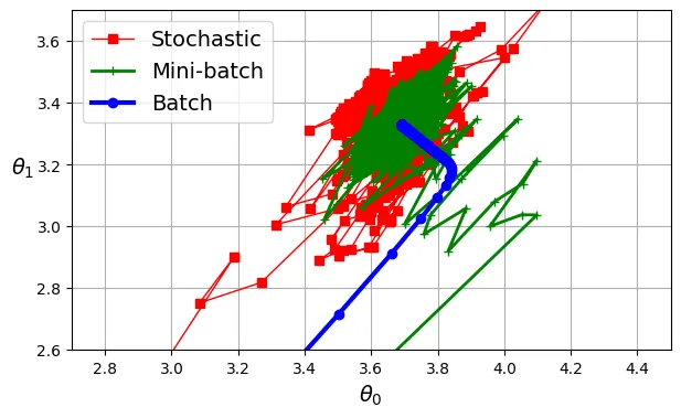
Biểu đồ không gian tham số cho thấy:
- Batch GD (xanh dương): Đi thẳng và ổn định đến đích nhưng tốn thời gian tính toán mỗi bước.
- Stochastic GD (đỏ): Nhảy loạn xạ nhưng đến đích rất nhanh, tuy nhiên không bao giờ đứng yên tại điểm tối ưu.
- Mini-batch GD (xanh lá): Ổn định hơn SGD và đến gần đích hơn Batch GD.
Hồi quy Đa thức (Polynomial Regression)
Khi dữ liệu có mối quan hệ phi tuyến, một đường thẳng sẽ không thể biểu diễn tốt (Underfitting). Giải pháp là thêm các đặc trưng đa thức (lũy thừa của đặc trưng gốc) vào dữ liệu, biến bài toán phi tuyến thành bài toán tuyến tính trong không gian đặc trưng mới.
Hãy thử tạo một dữ liệu tuân theo phương trình bậc hai: .
rng = np.random.default_rng(seed=42)
m = 200
X = 6 * rng.random((m, 1)) - 3
y = 0.5 * X ** 2 + X + 2 + rng.standard_normal((m, 1))

# đoạn code phụ – tạo Hình 4–12
plt.figure(figsize=(6, 4))
plt.plot(X, y, "b.")
plt.xlabel("$x_1$")
plt.ylabel("$y$", rotation=0)
plt.axis([-3, 3, 0, 10])
plt.grid()
plt.show()
Chúng ta sử dụng PolynomialFeatures để tạo đặc trưng .
from sklearn.preprocessing import PolynomialFeatures

# Tạo đặc trưng bậc 2, include_bias=False vì LinearRegression sẽ tự thêm bias
poly_features = PolynomialFeatures(degree=2, include_bias=False)
X_poly = poly_features.fit_transform(X)

X[0]
output:
array([1.64373629])X_poly[0]output:
array([1.64373629, 2.701869 ])X_poly bây giờ chứa đặc trưng gốc và bình phương của nó . Bây giờ ta có thể áp dụng LinearRegression như bình thường.
lin_reg = LinearRegression()
lin_reg.fit(X_poly, y)
lin_reg.intercept_, lin_reg.coef_
output:
(array([2.00540719]), array([[1.11022126, 0.50526985]]))Mô hình ước lượng: . Rất gần với thực tế (cộng nhiễu).
# đoạn code phụ – tạo Hình 4–13
X_new = np.linspace(-3, 3, 100).reshape(100, 1)
X_new_poly = poly_features.transform(X_new)
y_new = lin_reg.predict(X_new_poly)

plt.figure(figsize=(6, 4))
plt.plot(X, y, "b.")
plt.plot(X_new, y_new, "r-", linewidth=2, label="Predictions")
plt.xlabel("$x_1$")
plt.ylabel("$y$", rotation=0)
plt.legend(loc="upper left")
plt.axis([-3, 3, 0, 10])
plt.grid()
plt.show()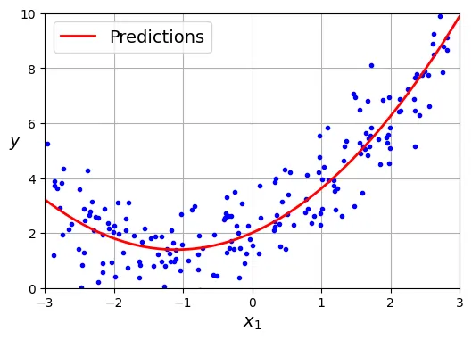
Đường cong Học tập (Learning Curves)
Một câu hỏi quan trọng: Chọn bậc đa thức bao nhiêu là đủ?
- Bậc quá thấp Underfitting (Bias cao).
- Bậc quá cao Overfitting (Variance cao).
Hình dưới đây minh họa điều này:
# đoạn code phụ – tạo Hình 4–14
from sklearn.preprocessing import StandardScaler
from sklearn.pipeline import make_pipeline

plt.figure(figsize=(6, 4))

# Vẽ 3 mô hình với các bậc đa thức khác nhau
for style, width, degree in (("r-+", 2, 1), ("b--", 2, 2), ("g-", 1, 300)):
    polybig_features = PolynomialFeatures(degree=degree, include_bias=False)
    std_scaler = StandardScaler()
    lin_reg = LinearRegression()
    polynomial_regression = make_pipeline(polybig_features, std_scaler, lin_reg)
    polynomial_regression.fit(X, y)
    y_newbig = polynomial_regression.predict(X_new)
    label = f"{degree} degree{'s' if degree > 1 else ''}"
    plt.plot(X_new, y_newbig, style, label=label, linewidth=width)

plt.plot(X, y, "b.", linewidth=3)
plt.legend(loc="upper left")
plt.xlabel("$x_1$")
plt.ylabel("$y$", rotation=0)
plt.axis([-3, 3, 0, 10])
plt.grid()
plt.show()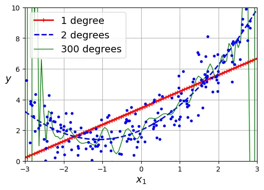
Để chẩn đoán mô hình, chúng ta sử dụng Learning Curves. Đường cong này vẽ sai số (RMSE) trên tập huấn luyện và tập kiểm định (validation set) theo kích thước của tập huấn luyện.
Đầu tiên, hãy xem đường cong của mô hình tuyến tính (Underfitting):
from sklearn.model_selection import learning_curve

train_sizes, train_scores, valid_scores = learning_curve(
    LinearRegression(), X, y, train_sizes=np.linspace(0.01, 1.0, 40), cv=5,
    scoring="neg_root_mean_squared_error")

# Đổi dấu vì scoring trả về giá trị âm (neg_root_mean_squared_error)
train_errors = -train_scores.mean(axis=1)
valid_errors = -valid_scores.mean(axis=1)

plt.figure(figsize=(6, 4))  # đoạn code phụ
plt.plot(train_sizes, train_errors, "r-+", linewidth=2, label="train")
plt.plot(train_sizes, valid_errors, "b-", linewidth=3, label="valid")

# đoạn code phụ – làm đẹp Hình 4–15
plt.xlabel("Training set size")
plt.ylabel("RMSE")
plt.grid()
plt.legend(loc="upper right")
plt.axis([0, 160, 0, 2.5])
plt.show()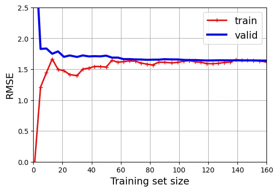
Dấu hiệu Underfitting:
- Lỗi trên tập train và valid đều cao.
- Chúng hội tụ nhanh chóng và đạt đến bình nguyên (plateau).
- Thêm dữ liệu không giúp giảm lỗi.
Tiếp theo, hãy xem đường cong của mô hình đa thức bậc 10 (Overfitting):
from sklearn.pipeline import make_pipeline

polynomial_regression = make_pipeline(
    PolynomialFeatures(degree=10, include_bias=False),
    LinearRegression())

train_sizes, train_scores, valid_scores = learning_curve(
    polynomial_regression, X, y, train_sizes=np.linspace(0.01, 1.0, 40), cv=5,
    scoring="neg_root_mean_squared_error")

# đoạn code phụ – tạo Hình 4–16
train_errors = -train_scores.mean(axis=1)
valid_errors = -valid_scores.mean(axis=1)

plt.figure(figsize=(6, 4))
plt.plot(train_sizes, train_errors, "r-+", linewidth=2, label="train")
plt.plot(train_sizes, valid_errors, "b-", linewidth=3, label="valid")
plt.legend(loc="upper right")
plt.xlabel("Training set size")
plt.ylabel("RMSE")
plt.grid()
plt.axis([0, 160, 0, 2.5])
plt.show()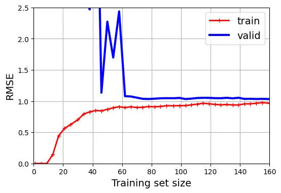
Dấu hiệu Overfitting:
- Lỗi trên tập train thấp hơn đáng kể so với tập valid.
- Có một khoảng cách (gap) lớn giữa hai đường.
- Khi tăng kích thước tập train, hai đường có xu hướng tiến lại gần nhau Cần thêm dữ liệu.
Mô hình Tuyến tính có Chính quy hóa (Regularized Linear Models)
Để giảm Overfitting, chúng ta sử dụng Chính quy hóa (Regularization): thêm một thành phần phạt vào hàm mất mát để hạn chế độ lớn của các trọng số .
Ridge Regression (Chuẩn )
Hàm mất mát của Ridge:
Siêu tham số kiểm soát mức độ chính quy hóa. là hồi quy tuyến tính thường. rất lớn thì các trọng số gần bằng 0 (đường dự đoán là đường thẳng ngang qua trung bình của y).
# đoạn code phụ – tạo dữ liệu nhiễu
rng = np.random.default_rng(seed=42)
m = 20  # số lượng mẫu ít
X = 3 * rng.random((m, 1))
y = 1 + 0.5 * X + rng.standard_normal((m, 1)) / 1.5
X_new = np.linspace(0, 3, 100).reshape(100, 1)

# đoạn code phụ – hiển thị dữ liệu
plt.figure(figsize=(6, 4))
plt.plot(X, y, ".")
plt.xlabel("$x_1$")
plt.ylabel("$y$  ", rotation=0)
plt.axis([0, 3, 0, 3.5])
plt.grid()
plt.show()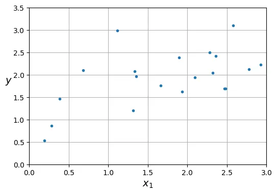
from sklearn.linear_model import Ridge

# Ridge Regression với solver Cholesky (dạng đóng)
ridge_reg = Ridge(alpha=0.1, solver="cholesky")
ridge_reg.fit(X, y)
ridge_reg.predict([[1.5]])
output:
array([1.84414523])Đoạn mã so sánh Ridge với các khác nhau:
# đoạn code phụ – tạo Hình 4–17
def plot_model(model_class, polynomial, alphas, **model_kwargs):
    plt.plot(X, y, "b.", linewidth=3)
    for alpha, style in zip(alphas, ("b:", "g--", "r-")):
        if alpha > 0:
            model = model_class(alpha, **model_kwargs)
        else:
            model = LinearRegression()
        if polynomial:
            model = make_pipeline(
                PolynomialFeatures(degree=10, include_bias=False),
                StandardScaler(),
                model)
        model.fit(X, y)
        y_new_regul = model.predict(X_new)
        plt.plot(X_new, y_new_regul, style, linewidth=2,
                 label=fr"$\alpha = {alpha}$")
    plt.legend(loc="upper left")
    plt.xlabel("$x_1$")
    plt.axis([0, 3, 0, 3.5])
    plt.grid()

plt.figure(figsize=(9, 3.5))
plt.subplot(121)
plot_model(Ridge, polynomial=False, alphas=(0, 10, 100), random_state=42)
plt.ylabel("$y$  ", rotation=0)

plt.subplot(122)
plot_model(Ridge, polynomial=True, alphas=(0, 10**-5, 1), random_state=42)
plt.gca().axes.yaxis.set_ticklabels([])
plt.show()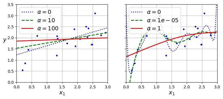
Bạn cũng có thể dùng SGD cho Ridge bằng cách đặt penalty="l2".
sgd_reg = SGDRegressor(penalty="l2", alpha=0.1 / m, tol=None,
                       max_iter=1000, eta0=0.01, random_state=42)
sgd_reg.fit(X, y.ravel())
sgd_reg.predict([[1.5]])
output:
array([1.83659707])Lasso Regression (Chuẩn )
Hàm mất mát của Lasso:
Lasso có tính chất quan trọng: Nó có xu hướng loại bỏ hoàn toàn các trọng số của các đặc trưng ít quan trọng (đưa về 0). Do đó, nó tự động thực hiện lựa chọn đặc trưng (feature selection) và tạo ra mô hình thưa (sparse model).
from sklearn.linear_model import Lasso

lasso_reg = Lasso(alpha=0.1)
lasso_reg.fit(X, y)
lasso_reg.predict([[1.5]])
output:
array([1.87550211])# đoạn code phụ – tạo Hình 4–18 minh họa Lasso
plt.figure(figsize=(9, 3.5))
plt.subplot(121)
plot_model(Lasso, polynomial=False, alphas=(0, 0.1, 1), random_state=42)
plt.ylabel("$y$ ", rotation=0)
plt.subplot(122)
plot_model(Lasso, polynomial=True, alphas=(0, 1e-2, 1), random_state=42)
plt.gca().axes.yaxis.set_ticklabels([])
plt.show()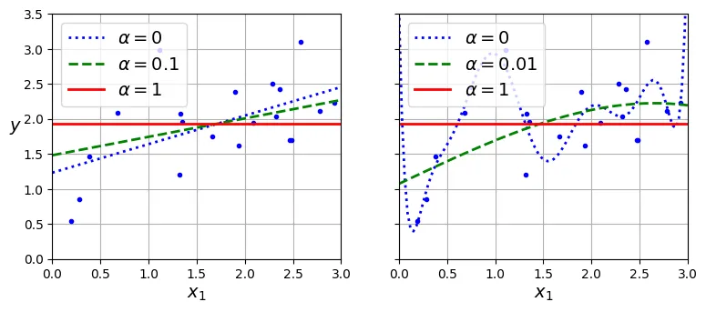
Elastic Net
Là sự kết hợp giữa Ridge và Lasso:
Tham số (l1_ratio) kiểm soát tỷ lệ pha trộn.
from sklearn.linear_model import ElasticNet

elastic_net = ElasticNet(alpha=0.1, l1_ratio=0.5)
elastic_net.fit(X, y)
elastic_net.predict([[1.5]])
output:
array([1.8645014])Early Stopping (Dừng sớm)
Thay vì thêm số hạng phạt, chúng ta có thể dừng quá trình huấn luyện (Gradient Descent) ngay khi sai số trên tập kiểm định đạt giá trị tối thiểu.
from copy import deepcopy
from sklearn.metrics import root_mean_squared_error
from sklearn.preprocessing import StandardScaler

# đoạn code phụ – tạo lại dữ liệu bậc 2 và chia train/valid
rng = np.random.default_rng(seed=42)
m = 200
X = 6 * rng.random((m, 1)) - 3
y = 0.5 * X ** 2 + X + 2 + rng.standard_normal((m, 1))
X_train, y_train = X[: m // 2], y[: m // 2, 0]
X_valid, y_valid = X[m // 2 :], y[m // 2 :, 0]

preprocessing = make_pipeline(PolynomialFeatures(degree=90, include_bias=False),
                              StandardScaler())
X_train_prep = preprocessing.fit_transform(X_train)
X_valid_prep = preprocessing.transform(X_valid)

sgd_reg = SGDRegressor(penalty=None, eta0=0.002, random_state=42)
n_epochs = 500
best_valid_rmse = float('inf')
train_errors, val_errors = [], []

for epoch in range(n_epochs):
    sgd_reg.partial_fit(X_train_prep, y_train)
    y_valid_predict = sgd_reg.predict(X_valid_prep)
    val_error = root_mean_squared_error(y_valid, y_valid_predict)

    # Lưu lại mô hình tốt nhất
    if val_error < best_valid_rmse:
        best_valid_rmse = val_error
        best_model = deepcopy(sgd_reg)

    # Tính toán lỗi huấn luyện để vẽ biểu đồ
    y_train_predict = sgd_reg.predict(X_train_prep)
    train_error = root_mean_squared_error(y_train, y_train_predict)
    val_errors.append(val_error)
    train_errors.append(train_error)

# đoạn code phụ – tạo Hình 4–20
best_epoch = np.argmin(val_errors)
plt.figure(figsize=(6, 4))
plt.annotate('Best model',
             xy=(best_epoch, best_valid_rmse),
             xytext=(best_epoch, best_valid_rmse + 0.5),
             ha="center",
             arrowprops=dict(facecolor='black', shrink=0.05))
plt.plot([0, n_epochs], [best_valid_rmse, best_valid_rmse], "k:", linewidth=2)
plt.plot(val_errors, "b-", linewidth=3, label="Validation set")
plt.plot(best_epoch, best_valid_rmse, "bo")
plt.plot(train_errors, "r--", linewidth=2, label="Training set")
plt.legend(loc="upper right")
plt.xlabel("Epoch")
plt.ylabel("RMSE")
plt.axis([0, n_epochs, 0, 3.5])
plt.grid()
plt.show()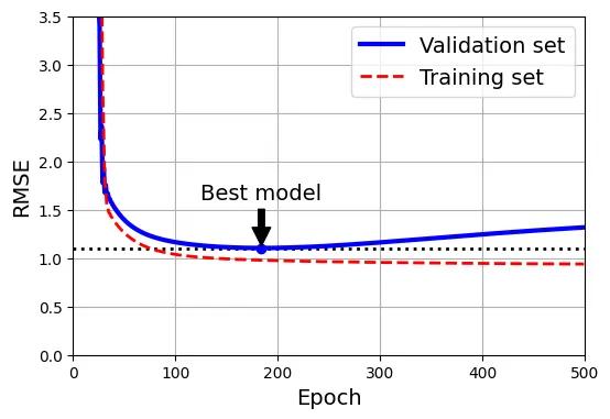
Hồi quy Logistic (Logistic Regression)
Hồi quy Logistic được dùng cho bài toán Phân loại (Classification), đặc biệt là ước tính xác suất.
Hàm Sigmoid
Mô hình tính toán điểm số , sau đó đưa qua hàm Sigmoid để nén giá trị vào khoảng [0, 1].
# đoạn code phụ – tạo Hình 4–21 minh họa hàm Sigmoid
lim = 6
t = np.linspace(-lim, lim, 100)
sig = 1 / (1 + np.exp(-t))

plt.figure(figsize=(8, 3))
plt.plot([-lim, lim], [0, 0], "k-")
plt.plot([-lim, lim], [0.5, 0.5], "k:")
plt.plot([-lim, lim], [1, 1], "k:")
plt.plot([0, 0], [-1.1, 1.1], "k-")
plt.plot(t, sig, "b-", linewidth=2, label=r"$\sigma(t) = \dfrac{1}{1 + e^{-t}}$")
plt.xlabel("t")
plt.legend(loc="upper left")
plt.axis([-lim, lim, -0.1, 1.1])
plt.gca().set_yticks([0, 0.25, 0.5, 0.75, 1])
plt.grid()
plt.show()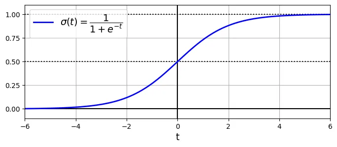
Ranh giới Quyết định (Decision Boundaries)
Sử dụng bộ dữ liệu Iris để minh họa.
from sklearn.datasets import load_iris

iris = load_iris(as_frame=True)
list(iris)
output:
['data',
'target',
'frame',
'target_names',
'DESCR',
'feature_names',
'filename',
'data_module']print(iris.DESCR) # Xem mô tả dữ liệuoutput:
.. _iris_dataset:
Iris plants dataset
--------------------
...iris.data.head(3)output:
sepal length (cm) sepal width (cm) petal length (cm) petal width (cm)
0 5.1 3.5 1.4 0.2
1 4.9 3.0 1.4 0.2
2 4.7 3.2 1.3 0.2iris.target.head(3) # Lưu ý dữ liệu chưa được xáo trộnoutput:
0 0
1 0
2 0
Name: target, dtype: int64iris.target_namesoutput:
array(['setosa', 'versicolor', 'virginica'], dtype='<U10')Huấn luyện mô hình để phát hiện loài Iris virginica dựa trên độ rộng cánh hoa.
from sklearn.linear_model import LogisticRegression
from sklearn.model_selection import train_test_split

X = iris.data[["petal width (cm)"]].values
y = iris.target_names[iris.target] == 'virginica'

X_train, X_test, y_train, y_test = train_test_split(X, y, random_state=42)

log_reg = LogisticRegression(random_state=42)
log_reg.fit(X_train, y_train)
output:
LogisticRegression(random_state=42)X_new = np.linspace(0, 3, 1000).reshape(-1, 1) # reshape thành cột vector
y_proba = log_reg.predict_proba(X_new)
decision_boundary = X_new[y_proba[:, 1] >= 0.5][0, 0]
plt.figure(figsize=(8, 3)) # đoạn code phụ
plt.plot(X_new, y_proba[:, 0], "b--", linewidth=2,
label="Not Iris virginica proba")
plt.plot(X_new, y_proba[:, 1], "g-", linewidth=2, label="Iris virginica proba")
plt.plot([decision_boundary, decision_boundary], [0, 1], "k:", linewidth=2,
label="Decision boundary")
# đoạn code phụ – làm đẹp Hình 4–23
plt.arrow(x=decision_boundary, y=0.08, dx=-0.3, dy=0,
head_width=0.05, head_length=0.1, fc="b", ec="b")
plt.arrow(x=decision_boundary, y=0.92, dx=0.3, dy=0,
head_width=0.05, head_length=0.1, fc="g", ec="g")
plt.plot(X_train[y_train == 0], y_train[y_train == 0], "bs")
plt.plot(X_train[y_train == 1], y_train[y_train == 1], "g^")
plt.xlabel("Petal width (cm)")
plt.ylabel("Probability")
plt.legend(loc="center left")
plt.axis([0, 3, -0.02, 1.02])
plt.grid()
plt.show()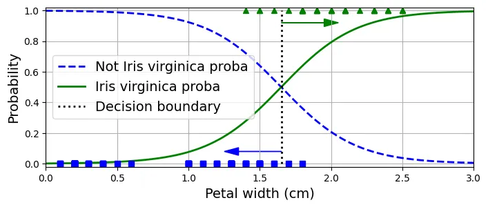
decision_boundaryoutput:
np.float64(1.6516516516516517)log_reg.predict([[1.7], [1.5]])output:
array([ True, False])Vùng quyết định 2D:
# đoạn code phụ – tạo Hình 4–24
X = iris.data[["petal length (cm)", "petal width (cm)"]].values
y = iris.target_names[iris.target] == 'virginica'
X_train, X_test, y_train, y_test = train_test_split(X, y, random_state=42)

log_reg = LogisticRegression(C=2, random_state=42)
log_reg.fit(X_train, y_train)

# cho biểu đồ đường đồng mức (contour plot)
x0, x1 = np.meshgrid(np.linspace(2.9, 7, 500).reshape(-1, 1),
                     np.linspace(0.8, 2.7, 200).reshape(-1, 1))
X_new = np.c_[x0.ravel(), x1.ravel()]
y_proba = log_reg.predict_proba(X_new)
zz = y_proba[:, 1].reshape(x0.shape)

# cho đường ranh giới quyết định
left_right = np.array([2.9, 7])
boundary = -((log_reg.coef_[0, 0] * left_right + log_reg.intercept_[0])
             / log_reg.coef_[0, 1])

plt.figure(figsize=(10, 4))
plt.plot(X_train[y_train == 0, 0], X_train[y_train == 0, 1], "bs")
plt.plot(X_train[y_train == 1, 0], X_train[y_train == 1, 1], "g^")
contour = plt.contour(x0, x1, zz, cmap=plt.cm.brg)
plt.clabel(contour, inline=1)
plt.plot(left_right, boundary, "k--", linewidth=3)
plt.text(3.5, 1.27, "Not Iris virginica", color="b", ha="center")
plt.text(6.5, 2.3, "Iris virginica", color="g", ha="center")
plt.xlabel("Petal length")
plt.ylabel("Petal width")
plt.axis([2.9, 7, 0.8, 2.7])
plt.grid()
plt.show()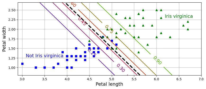
Softmax Regression
Tổng quát hóa Logistic Regression cho bài toán đa lớp. Sử dụng hàm Softmax để tính xác suất cho từng lớp.
X = iris.data[["petal length (cm)", "petal width (cm)"]].values
y = iris["target"]
X_train, X_test, y_train, y_test = train_test_split(X, y, random_state=42)

# C=30 là nghịch đảo của alpha (regularization), C càng lớn -> regularization càng ít
softmax_reg = LogisticRegression(C=30, random_state=42)
softmax_reg.fit(X_train, y_train)
output:
LogisticRegression(C=30, random_state=42)softmax_reg.predict([[5, 2]])output:
array([2])softmax_reg.predict_proba([[5, 2]]).round(2)output:
array([[0. , 0.04, 0.96]])# đoạn code phụ – tạo Hình 4–25
from matplotlib.colors import ListedColormap
custom_cmap = ListedColormap(["#fafab0", "#9898ff", "#a0faa0"])
x0, x1 = np.meshgrid(np.linspace(0, 8, 500).reshape(-1, 1),
np.linspace(0, 3.5, 200).reshape(-1, 1))
X_new = np.c_[x0.ravel(), x1.ravel()]
y_proba = softmax_reg.predict_proba(X_new)
y_predict = softmax_reg.predict(X_new)
zz1 = y_proba[:, 1].reshape(x0.shape)
zz = y_predict.reshape(x0.shape)
plt.figure(figsize=(10, 4))
plt.plot(X[y == 2, 0], X[y == 2, 1], "g^", label="Iris virginica")
plt.plot(X[y == 1, 0], X[y == 1, 1], "bs", label="Iris versicolor")
plt.plot(X[y == 0, 0], X[y == 0, 1], "yo", label="Iris setosa")
plt.contourf(x0, x1, zz, cmap=custom_cmap)
contour = plt.contour(x0, x1, zz1, cmap="hot")
plt.clabel(contour, inline=1)
plt.xlabel("Petal length")
plt.ylabel("Petal width")
plt.legend(loc="center left")
plt.axis([0.5, 7, 0, 3.5])
plt.grid()
plt.show()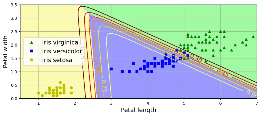
Ôn tập
1. Thuật toán GD nào phù hợp cho hàng triệu đặc trưng? Stochastic Gradient Descent (SGD) hoặc Mini-batch GD. Phương trình Pháp tuyến không dùng được vì độ phức tạp đến .
2. Nếu các đặc trưng có tỉ lệ khác nhau? Gradient Descent sẽ hội tụ rất chậm (hình cái bát kéo dài). Cần chuẩn hóa dữ liệu (StandardScaler).
3. GD có bị mắc kẹt ở cực tiểu địa phương với Logistic Regression không? Không, vì hàm mất mát của Logistic Regression là hàm lồi (convex).
4. Tất cả GD có hội tụ về cùng một điểm không? Nếu learning rate đủ nhỏ, chúng sẽ hội tụ về cùng một vùng. Batch GD hội tụ chính xác, SGD và Mini-batch sẽ dao động quanh điểm tối ưu.
5. Validation error tăng liên tục? Nếu training error cũng tăng Learning rate quá cao. Nếu training error giảm Overfitting (dừng sớm).
Bài tập thực hành: Cài đặt Batch Gradient Descent với Early Stopping cho Softmax Regression
Tự cài đặt Softmax Regression bằng NumPy.
X = iris.data[["petal length (cm)", "petal width (cm)"]].values
y = iris["target"].values
Thêm bias term:
X_with_bias = np.c_[np.ones(len(X)), X]Chia tập dữ liệu thủ công:
test_ratio = 0.2
validation_ratio = 0.2
total_size = len(X_with_bias)

test_size = int(total_size * test_ratio)
validation_size = int(total_size * validation_ratio)
train_size = total_size - test_size - validation_size

rng = np.random.default_rng(seed=42)
rnd_indices = rng.permutation(total_size)

X_train = X_with_bias[rnd_indices[:train_size]]
y_train = y[rnd_indices[:train_size]]
X_valid = X_with_bias[rnd_indices[train_size:-test_size]]
y_valid = y[rnd_indices[train_size:-test_size]]
X_test = X_with_bias[rnd_indices[-test_size:]]
y_test = y[rnd_indices[-test_size:]]
One-hot Encoding:
def to_one_hot(y):
    return np.diag(np.ones(y.max() + 1))[y]

Y_train_one_hot = to_one_hot(y_train)
Y_valid_one_hot = to_one_hot(y_valid)
Y_test_one_hot = to_one_hot(y_test)
Chuẩn hóa dữ liệu:
mean = X_train[:, 1:].mean(axis=0)
std = X_train[:, 1:].std(axis=0)

X_train[:, 1:] = (X_train[:, 1:] - mean) / std
X_valid[:, 1:] = (X_valid[:, 1:] - mean) / std
X_test[:, 1:] = (X_test[:, 1:] - mean) / std
Hàm Softmax:
def softmax(logits):
    exps = np.exp(logits)
    exp_sums = exps.sum(axis=1, keepdims=True)
    return exps / exp_sums
Huấn luyện với Cross Entropy Loss:
n_inputs = X_train.shape[1]
n_outputs = len(np.unique(y_train))
eta = 0.5
n_epochs = 5001
m = len(X_train)
epsilon = 1e-5

rng = np.random.default_rng(seed=42)
Theta = rng.standard_normal((n_inputs, n_outputs))

for epoch in range(n_epochs):
    logits = X_train @ Theta
    Y_proba = softmax(logits)
    if epoch % 1000 == 0:
        Y_proba_valid = softmax(X_valid @ Theta)
        xentropy_losses = -(Y_valid_one_hot * np.log(Y_proba_valid + epsilon))
        print(epoch, xentropy_losses.sum(axis=1).mean())
    error = Y_proba - Y_train_one_hot
    gradients = 1 / m * X_train.T @ error
    Theta = Theta - eta * gradients
output:
0 2.973977344302766
1000 0.09313918303944396
2000 0.0890469894612578
3000 0.08847558719791132
4000 0.08861927669821175
5000 0.08894346006981158Đánh giá:
logits = X_valid @ Theta
Y_proba = softmax(logits)
y_predict = Y_proba.argmax(axis=1)
accuracy_score = (y_predict == y_valid).mean()
accuracy_score
output:
np.float64(0.9333333333333333)Thêm L2 Regularization:
eta = 0.5
n_epochs = 5001
m = len(X_train)
epsilon = 1e-5
alpha = 0.01

rng = np.random.default_rng(seed=42)
Theta = rng.standard_normal((n_inputs, n_outputs))

for epoch in range(n_epochs):
    logits = X_train @ Theta
    Y_proba = softmax(logits)
    if epoch % 1000 == 0:
        Y_proba_valid = softmax(X_valid @ Theta)
        xentropy_losses = -(Y_valid_one_hot * np.log(Y_proba_valid + epsilon))
        l2_loss = 1 / 2 * (Theta[1:] ** 2).sum()
        total_loss = xentropy_losses.sum(axis=1).mean() + alpha * l2_loss
        print(epoch, total_loss.round(4))
    error = Y_proba - Y_train_one_hot
    gradients = 1 / m * X_train.T @ error
    gradients += np.r_[np.zeros([1, n_outputs]), alpha * Theta[1:]]
    Theta = Theta - eta * gradients
output:
0 3.0065
1000 0.2711
2000 0.2711
3000 0.2711
4000 0.2711
5000 0.2711logits = X_valid @ Theta
Y_proba = softmax(logits)
y_predict = Y_proba.argmax(axis=1)
accuracy_score = (y_predict == y_valid).mean()
accuracy_scoreoutput:
np.float64(0.9666666666666667)Thêm Early Stopping:
eta = 0.5
n_epochs = 50_001
m = len(X_train)
epsilon = 1e-5
C = 100
best_loss = np.inf

rng = np.random.default_rng(seed=42)
Theta = rng.standard_normal((n_inputs, n_outputs))

for epoch in range(n_epochs):
    logits = X_train @ Theta
    Y_proba = softmax(logits)
    Y_proba_valid = softmax(X_valid @ Theta)
    xentropy_losses = -(Y_valid_one_hot * np.log(Y_proba_valid + epsilon))
    l2_loss = 1 / 2 * (Theta[1:] ** 2).sum()
    total_loss = xentropy_losses.sum(axis=1).mean() + 1 / C * l2_loss

    if epoch % 1000 == 0:
        print(epoch, total_loss.round(4))

    if total_loss < best_loss:
        best_loss = total_loss
    else:
        print(epoch - 1, best_loss.round(4))
        print(epoch, total_loss.round(4), "early stopping!")
        break

    error = Y_proba - Y_train_one_hot
    gradients = 1 / m * X_train.T @ error
    gradients += np.r_[np.zeros([1, n_outputs]), 1 / C * Theta[1:]]
    Theta = Theta - eta * gradients
output:
0 3.0065
402 0.2711
403 0.2711 early stopping!logits = X_valid @ Theta
Y_proba = softmax(logits)
y_predict = Y_proba.argmax(axis=1)
accuracy_score = (y_predict == y_valid).mean()
accuracy_scoreoutput:
np.float64(0.9666666666666667)Trực quan hóa:
custom_cmap = mpl.colors.ListedColormap(['#fafab0', '#9898ff', '#a0faa0'])
x0, x1 = np.meshgrid(np.linspace(0, 8, 500).reshape(-1, 1),
                     np.linspace(0, 3.5, 200).reshape(-1, 1))
X_new = np.c_[x0.ravel(), x1.ravel()]
X_new = (X_new - mean) / std
X_new_with_bias = np.c_[np.ones(len(X_new)), X_new]

logits = X_new_with_bias @ Theta
Y_proba = softmax(logits)
y_predict = Y_proba.argmax(axis=1)

zz1 = Y_proba[:, 1].reshape(x0.shape)
zz = y_predict.reshape(x0.shape)

plt.figure(figsize=(10, 4))
plt.plot(X[y == 2, 0], X[y == 2, 1], "g^", label="Iris virginica")
plt.plot(X[y == 1, 0], X[y == 1, 1], "bs", label="Iris versicolor")
plt.plot(X[y == 0, 0], X[y == 0, 1], "yo", label="Iris setosa")
plt.contourf(x0, x1, zz, cmap=custom_cmap)
contour = plt.contour(x0, x1, zz1, cmap="hot")
plt.clabel(contour, inline=1)
plt.xlabel("Petal length")
plt.ylabel("Petal width")
plt.legend(loc="upper left")
plt.axis([0, 7, 0, 3.5])
plt.grid()
plt.show()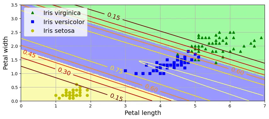
logits = X_test @ Theta
Y_proba = softmax(logits)
y_predict = Y_proba.argmax(axis=1)
accuracy_score = (y_predict == y_test).mean()
accuracy_score
output:
np.float64(0.9666666666666667)