[ML101] Chương 3: Bài toán Phân loại (Classification)
Tìm hiểu về bài toán phân loại trong Machine Learning với các thuật toán phổ biến
Bài viết có tham khảo, sử dụng và sửa đổi tài nguyên từ kho lưu trữ handson-mlp, tuân thủ giấy phép Apache‑2.0. Chúng tôi chân thành cảm ơn tác giả Aurélien Géron (@aureliengeron) vì sự chia sẻ kiến thức tuyệt vời và những đóng góp quý giá cho cộng đồng.
Chào mừng bạn đến với Chương 3.
Trong chương trước, chúng ta đã tiếp cận bài toán Hồi quy (Regression), nơi mục tiêu là dự đoán một giá trị thực liên tục . Trong chương này, chúng ta sẽ chuyển sang một nhiệm vụ khác: Phân loại (Classification). Tại đây, biến mục tiêu là một biến rời rạc, thuộc về một tập hữu hạn các nhãn lớp (class labels).
Chúng ta sẽ xây dựng các mô hình từ cơ bản như Phân loại Nhị phân (Binary Classification - ) đến phức tạp hơn như Phân loại Đa lớp (Multiclass), Đa nhãn (Multilabel) và Đa đầu ra (Multioutput).
Bạn có thể chạy trực tiếp các đoạn mã code tại: Google Colab.
Cài đặt môi trường
Để đảm bảo tính nhất quán và khả năng tái lập (reproducibility) của các thí nghiệm, việc kiểm soát phiên bản phần mềm là nên làm. Các thuật toán và API trong Machine Learning thay đổi thường xuyên; do đó, chúng ta cần xác nhận môi trường thực thi đáp ứng đúng yêu cầu.
Đoạn mã dưới đây kiểm tra phiên bản Python. Chúng ta yêu cầu Python 3.10+ để tận dụng các tính năng mới về type hinting và tối ưu hóa hiệu năng:
import sys

# Kiểm tra xem phiên bản Python có lớn hơn hoặc bằng 3.10 không
assert sys.version_info >= (3, 10)
Tiếp theo, chúng ta kiểm tra thư viện Scikit-Learn (sklearn). Đây là thư viện thông dụng cho các thuật toán Machine Learning cổ điển. Phiên bản 1.6.1 được yêu cầu để đảm bảo các hàm như LinearRegression hay KNeighborsRegressor hoạt động chính xác như trong Chương này.
from packaging.version import Version
import sklearn

# Kiểm tra phiên bản của thư viện Scikit-Learn
assert Version(sklearn.__version__) >= Version("1.6.1")
Chúng ta cũng thiết lập cấu hình cho Matplotlib để đảm bảo các biểu đồ hiển thị rõ ràng, hỗ trợ việc phân tích định lượng trên đồ thị.
import matplotlib.pyplot as plt

# Thiết lập kích thước phông chữ chung là 12
plt.rc('font', size=12)
# Thiết lập kích thước phông chữ cho nhãn trục (x, y) là 14
plt.rc('axes', labelsize=14, titlesize=14)
# Thiết lập kích thước phông chữ cho chú thích (legend) là 12
plt.rc('legend', fontsize=12)
# Thiết lập kích thước phông chữ cho các vạch chia trên trục x và y là 10
plt.rc('xtick', labelsize=10)
plt.rc('ytick', labelsize=10)
Bộ dữ liệu MNIST
Chúng ta sẽ sử dụng bộ dữ liệu MNIST (Modified National Institute of Standards and Technology). Trong cộng đồng thị giác máy tính (Computer Vision), MNIST đóng vai trò như “Hello World”. Nó bao gồm 70,000 ảnh xám (grayscale) kích thước pixel, biểu diễn các chữ số viết tay từ 0 đến 9.
Hàm fetch_openml cho phép tải dữ liệu trực tiếp từ kho lưu trữ OpenML. Tham số as_frame=False được sử dụng để dữ liệu trả về dưới dạng mảng NumPy (tối ưu cho tính toán ma trận) thay vì Pandas DataFrame.
from sklearn.datasets import fetch_openml

# Tải bộ dữ liệu MNIST từ OpenML
# as_frame=False để trả về dạng mảng NumPy thay vì DataFrame của Pandas
mnist = fetch_openml('mnist_784', as_frame=False)
Dữ liệu đi kèm với siêu dữ liệu (metadata) mô tả nguồn gốc và cấu trúc. Việc đọc kỹ mô tả này giúp chúng ta hiểu về phân phối và quy trình thu thập dữ liệu gốc.
# extra code – đoạn này chỉ để in ra mô tả, hơi dài một chút
print(mnist.DESCR)
output:
**Author**: Yann LeCun, Corinna Cortes, Christopher J.C. Burges
**Source**: [MNIST Website](http://yann.lecun.com/exdb/mnist/) - Date unknown
**Please cite**:
The MNIST database of handwritten digits with 784 features, raw data available at: http://yann.lecun.com/exdb/mnist/. It can be split in a training set of the first 60,000 examples, and a test set of 10,000 examples
It is a subset of a larger set available from NIST. The digits have been size-normalized and centered in a fixed-size image. It is a good database for people who want to try learning techniques and pattern recognition methods on real-world data while spending minimal efforts on preprocessing and formatting. The original black and white (bilevel) images from NIST were size normalized to fit in a 20x20 pixel box while preserving their aspect ratio. The resulting images contain grey levels as a result of the anti-aliasing technique used by the normalization algorithm. the images were centered in a 28x28 image by computing the center of mass of the pixels, and translating the image so as to position this point at the center of the 28x28 field.
With some classification methods (particularly template-based methods, such as SVM and K-nearest neighbors), the error rate improves when the digits are centered by bounding box rather than center of mass. If you do this kind of pre-processing, you should report it in your publications. The MNIST database was constructed from NIST's NIST originally designated SD-3 as their training set and SD-1 as their test set. However, SD-3 is much cleaner and easier to recognize than SD-1. The reason for this can be found on the fact that SD-3 was collected among Census Bureau employees, while SD-1 was collected among high-school students. Drawing sensible conclusions from learning experiments requires that the result be independent of the choice of training set and test among the complete set of samples. Therefore it was necessary to build a new database by mixing NIST's datasets.
The MNIST training set is composed of 30,000 patterns from SD-3 and 30,000 patterns from SD-1. Our test set was composed of 5,000 patterns from SD-3 and 5,000 patterns from SD-1. The 60,000 pattern training set contained examples from approximately 250 writers. We made sure that the sets of writers of the training set and test set were disjoint. SD-1 contains 58,527 digit images written by 500 different writers. In contrast to SD-3, where blocks of data from each writer appeared in sequence, the data in SD-1 is scrambled. Writer identities for SD-1 is available and we used this information to unscramble the writers. We then split SD-1 in two: characters written by the first 250 writers went into our new training set. The remaining 250 writers were placed in our test set. Thus we had two sets with nearly 30,000 examples each. The new training set was completed with enough examples from SD-3, starting at pattern # 0, to make a full set of 60,000 training patterns. Similarly, the new test set was completed with SD-3 examples starting at pattern # 35,000 to make a full set with 60,000 test patterns. Only a subset of 10,000 test images (5,000 from SD-1 and 5,000 from SD-3) is available on this site. The full 60,000 sample training set is available.
Downloaded from openml.org.Cấu trúc dữ liệu trả về là một dictionary. Chúng ta sẽ trích xuất ma trận đặc trưng và vector nhãn .
mnist.keys() # extra code – chúng ta chỉ quan tâm đến 'data' và 'target' trong notebook nàyoutput:
dict_keys(['data', 'target', 'frame', 'categories', 'feature_names', 'target_names', 'DESCR', 'details', 'url'])Mỗi hình ảnh được làm phẳng (flattened) từ ma trận 2D thành vector 1D có kích thước 784.
X, y = mnist.data, mnist.target
X
output:
array([[0, 0, 0, ..., 0, 0, 0],
[0, 0, 0, ..., 0, 0, 0],
[0, 0, 0, ..., 0, 0, 0],
...,
[0, 0, 0, ..., 0, 0, 0],
[0, 0, 0, ..., 0, 0, 0],
[0, 0, 0, ..., 0, 0, 0]])Kiểm tra chiều (shape) của dữ liệu là bước quan trọng trong Đại số tuyến tính để đảm bảo tính tương thích của các phép nhân ma trận sau này.
- : 70,000 mẫu, 784 đặc trưng.
- : 70,000 nhãn tương ứng.
X.shapeoutput:
(70000, 784)Vector nhãn hiện đang được lưu trữ dưới dạng chuỗi (string/object). Trong quá trình huấn luyện, hầu hết các thuật toán sẽ tự động chuyển đổi sang dạng số, nhưng nhận biết điều này giúp ta tránh các lỗi so sánh không mong muốn.
youtput:
array(['5', '0', '4', ..., '4', '5', '6'], dtype=object)y.shapeoutput:
(70000,)28 * 28output:
784Để con người có thể hiểu được dữ liệu, ta cần tái cấu trúc vector 784 chiều thành ma trận ảnh và hiển thị nó.
import matplotlib.pyplot as plt

def plot_digit(image_data):
    image = image_data.reshape(28, 28) # Chuyển mảng 1 chiều 784 thành ma trận 28x28
    plt.imshow(image, cmap="binary")   # Vẽ ảnh đen trắng (binary colormap)
    plt.axis("off")                    # Tắt trục tọa độ

some_digit = X[0]  # Lấy mẫu đầu tiên
plot_digit(some_digit)
plt.show()
Nhãn thực tế của hình ảnh trên:
y[0]output:
'5'Trực quan hóa một tập hợp các mẫu ngẫu nhiên giúp ta cảm nhận được độ biến thiên (variance) trong cách viết tay của con người (nét đậm, nhạt, nghiêng, xoay).
# extra code – đoạn mã này tạo ra Hình 3–2
plt.figure(figsize=(9, 9))
for idx, image_data in enumerate(X[:100]):
    plt.subplot(10, 10, idx + 1) # Tạo lưới 10x10
    plot_digit(image_data)
plt.subplots_adjust(wspace=0, hspace=0)
plt.show()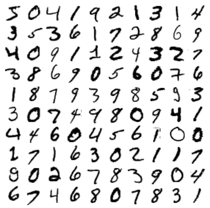
Chia tập dữ liệu (Train/Test Split): Việc chia tách dữ liệu là bắt buộc để đánh giá khả năng tổng quát hóa (generalization) của mô hình và tránh hiện tượng quá khớp (overfitting). MNIST đã được sắp xếp sao cho 60,000 mẫu đầu là huấn luyện và 10,000 mẫu sau là kiểm tra.
# Chia tập train (60k mẫu đầu) và test (10k mẫu sau)
X_train, X_test, y_train, y_test = X[:60000], X[60000:], y[:60000], y[60000:]
Huấn luyện Bộ phân loại Nhị phân (Binary Classifier)
Chúng ta sẽ đơn giản hóa bài toán thành: Xác định xem một chữ số có phải là số 5 hay không. Về mặt toán học, ta ánh xạ nhãn sang tập (hoặc ):
y_train_5 = (y_train == '5')  # True cho tất cả các số 5, False cho các số khác
y_test_5 = (y_test == '5')
Chúng ta sử dụng Stochastic Gradient Descent (SGD). Đây là một thuật toán tối ưu hóa lặp lại. Đối với phân loại tuyến tính (như SVM tuyến tính hoặc Logistic Regression), bộ phân loại tính toán điểm số . Nếu , dự đoán là lớp dương.
Trong Scikit-Learn, SGDClassifier mặc định triển khai thuật toán SVM tuyến tính (với hàm mất mát Hinge Loss). Tham số random_state=42 được thiết lập để cố định hạt giống ngẫu nhiên, đảm bảo kết quả huấn luyện là nhất quán qua các lần chạy.
from sklearn.linear_model import SGDClassifier

# Khởi tạo bộ phân loại SGD với random_state cố định để kết quả có thể tái lập
sgd_clf = SGDClassifier(random_state=42)
# Huấn luyện mô hình trên tập train
sgd_clf.fit(X_train, y_train_5)
output:
SGDClassifier(random_state=42)Thử nghiệm dự đoán trên mẫu some_digit (số 5):
sgd_clf.predict([some_digit])output:
array([ True])Các thước đo Hiệu năng (Performance Measures)
Trong phân loại, “Độ chính xác” (Accuracy) thường không đủ để đánh giá mô hình, đặc biệt khi dữ liệu bị mất cân bằng (imbalanced data).
Đo độ chính xác bằng Kiểm định chéo (Cross-Validation)
Kiểm định chéo K-fold (K-fold Cross-Validation) chia tập huấn luyện thành phần. Mô hình được huấn luyện trên phần và kiểm tra trên phần còn lại. Quy trình lặp lại lần.
Accuracy được tính bằng công thức:
from sklearn.model_selection import cross_val_score

# Đánh giá mô hình bằng accuracy (độ chính xác) với 3-fold cross-validation
cross_val_score(sgd_clf, X_train, y_train_5, cv=3, scoring="accuracy")
output:
array([0.95035, 0.96035, 0.9604 ])Để hiểu rõ cơ chế, đoạn mã dưới đây cài đặt thủ công StratifiedKFold. Phương pháp này đảm bảo tỷ lệ các lớp trong mỗi fold xấp xỉ tỷ lệ của tập dữ liệu gốc, giúp đánh giá ổn định hơn.
from sklearn.model_selection import StratifiedKFold
from sklearn.base import clone

skfolds = StratifiedKFold(n_splits=3)  # Thêm shuffle=True nếu dữ liệu chưa được xáo trộn

# Duyệt qua từng fold
for train_index, test_index in skfolds.split(X_train, y_train_5):
    clone_clf = clone(sgd_clf) # Sao chép mô hình gốc

    # Tách dữ liệu theo index
    X_train_folds = X_train[train_index]
    y_train_folds = y_train_5[train_index]
    X_test_fold = X_train[test_index]
    y_test_fold = y_train_5[test_index]

    # Huấn luyện và dự đoán
    clone_clf.fit(X_train_folds, y_train_folds)
    y_pred = clone_clf.predict(X_test_fold)

    # Tính tỷ lệ dự đoán đúng
    n_correct = sum(y_pred == y_test_fold)
    print(n_correct / len(y_pred))
output:
0.95035
0.96035
0.9604Tại sao Accuracy > 95% nhưng vẫn cần cảnh giác? Vì chỉ có khoảng 10% ảnh là số 5. Một mô hình “ngây thơ” luôn đoán “Không phải số 5” cũng sẽ đạt độ chính xác 90%. Đây là Nghịch lý về độ chính xác (Accuracy Paradox).
from sklearn.dummy import DummyClassifier

dummy_clf = DummyClassifier()
dummy_clf.fit(X_train, y_train_5)
print(any(dummy_clf.predict(X_train))) # Kiểm tra xem có dự đoán nào là True không
output:
False# Đánh giá Dummy Classifier
cross_val_score(dummy_clf, X_train, y_train_5, cv=3, scoring="accuracy")output:
array([0.90965, 0.90965, 0.90965])Ma trận Nhầm lẫn (Confusion Matrix)
Ma trận nhầm lẫn cung cấp cái nhìn chi tiết hơn về hiệu suất. Với bài toán nhị phân, ma trận có dạng:
Trong đó:
- TN (True Negative): Đúng là không phải 5.
- FP (False Positive): Nhầm là 5 (Lỗi loại I).
- FN (False Negative): Bỏ sót số 5 (Lỗi loại II).
- TP (True Positive): Đúng là số 5.
Ta dùng cross_val_predict để lấy dự đoán “sạch” (out-of-sample) cho từng mẫu trong tập huấn luyện.
from sklearn.model_selection import cross_val_predict

# Trả về kết quả dự đoán trên từng fold thay vì điểm số
y_train_pred = cross_val_predict(sgd_clf, X_train, y_train_5, cv=3)
from sklearn.metrics import confusion_matrix
cm = confusion_matrix(y_train_5, y_train_pred)
cmoutput:
array([[53892, 687],
[ 1891, 3530]])Một mô hình hoàn hảo sẽ có và .
y_train_perfect_predictions = y_train_5  # Giả sử chúng ta dự đoán đúng hoàn toàn
confusion_matrix(y_train_5, y_train_perfect_predictions)
output:
array([[54579, 0],
[ 0, 5421]])Precision và Recall
Từ ma trận nhầm lẫn, ta tính được các chỉ số quan trọng hơn:
-
Precision (Độ chính xác của dự báo dương): Trong các mẫu được dự đoán là 5, bao nhiêu % là đúng?
-
Recall (Độ phủ/Độ nhạy): Trong các mẫu thực sự là 5, bao nhiêu % được phát hiện?
from sklearn.metrics import precision_score, recall_score

precision_score(y_train_5, y_train_pred)  # Tương đương 3530 / (687 + 3530)
output:
0.8370879772350012# extra code – tính thủ công để kiểm chứng: TP / (FP + TP)
cm[1, 1] / (cm[0, 1] + cm[1, 1])output:
0.8370879772350012recall_score(y_train_5, y_train_pred) # Tương đương 3530 / (1891 + 3530)output:
0.6511713705958311# extra code – tính thủ công để kiểm chứng: TP / (FN + TP)
cm[1, 1] / (cm[1, 0] + cm[1, 1])output:
0.6511713705958311F1 Score là trung bình điều hòa (harmonic mean) của Precision và Recall, dùng để so sánh hai mô hình chỉ bằng một con số duy nhất. F1 ưu tiên sự cân bằng, nó sẽ thấp nếu một trong hai chỉ số kia thấp.
from sklearn.metrics import f1_score

f1_score(y_train_5, y_train_pred)
output:
0.7325171197343847# extra code – tính thủ công F1 score
cm[1, 1] / (cm[1, 1] + (cm[1, 0] + cm[0, 1]) / 2)output:
0.7325171197343847Sự đánh đổi giữa Precision và Recall (Precision/Recall Trade-off)
SGDClassifier tính toán một điểm số (decision score) cho mỗi mẫu.
Thay đổi threshold (ngưỡng) sẽ làm thay đổi Precision và Recall theo hướng ngược nhau. Tăng ngưỡng làm tăng Precision (khắt khe hơn) nhưng giảm Recall (bỏ sót nhiều hơn).
y_scores = sgd_clf.decision_function([some_digit])
y_scores
output:
array([2164.22030239])threshold = 0
y_some_digit_pred = (y_scores > threshold)
y_some_digit_predoutput:
array([ True])# extra code – minh họa rằng y_scores > 0 cho kết quả giống hàm predict()
y_scores > 0output:
array([ True])Nếu tăng ngưỡng lên 3000:
threshold = 3000
y_some_digit_pred = (y_scores > threshold)
y_some_digit_pred
output:
array([False])Để chọn ngưỡng tối ưu, chúng ta cần xem xét đường cong Precision-Recall trên toàn bộ tập dữ liệu.
y_scores = cross_val_predict(sgd_clf, X_train, y_train_5, cv=3,
                             method="decision_function")
from sklearn.metrics import precision_recall_curve
precisions, recalls, thresholds = precision_recall_curve(y_train_5, y_scores)Biểu đồ dưới đây minh họa sự biến thiên của Precision và Recall khi ngưỡng thay đổi.
plt.figure(figsize=(8, 4))  # extra code – định dạng hình ảnh
plt.plot(thresholds, precisions[:-1], "b--", label="Precision", linewidth=2)
plt.plot(thresholds, recalls[:-1], "g-", label="Recall", linewidth=2)
plt.vlines(threshold, 0, 1.0, "k", "dotted", label="threshold")

# extra code – trang trí cho Hình 3–5 thêm đẹp và dễ hiểu
idx = (thresholds >= threshold).argmax()  # tìm index đầu tiên >= threshold
plt.plot(thresholds[idx], precisions[idx], "bo")
plt.plot(thresholds[idx], recalls[idx], "go")
plt.axis([-50000, 50000, 0, 1])
plt.grid()
plt.xlabel("Threshold")
plt.legend(loc="center right")
plt.show()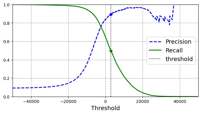
Biểu đồ Precision vs. Recall trực quan hơn để thấy sự đánh đổi.
import matplotlib.patches as patches  # extra code – dùng để vẽ mũi tên cong

plt.figure(figsize=(6, 5))  # extra code
plt.plot(recalls, precisions, linewidth=2, label="Precision/Recall curve")

# extra code – trang trí cho Hình 3–6
plt.plot([recalls[idx], recalls[idx]], [0., precisions[idx]], "k:")
plt.plot([0.0, recalls[idx]], [precisions[idx], precisions[idx]], "k:")
plt.plot([recalls[idx]], [precisions[idx]], "ko",
         label="Point at threshold 3,000")
plt.gca().add_patch(patches.FancyArrowPatch(
    (0.79, 0.60), (0.61, 0.78),
    connectionstyle="arc3,rad=.2",
    arrowstyle="Simple, tail_width=1.5, head_width=8, head_length=10",
    color="#444444"))
plt.text(0.56, 0.62, "Higher\nthreshold", color="#333333")
plt.xlabel("Recall")
plt.ylabel("Precision")
plt.axis([0, 1, 0, 1])
plt.grid()
plt.legend(loc="lower left")
plt.show()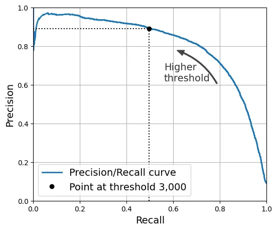
Nếu dự án yêu cầu Precision ít nhất 90%, ta có thể tìm ngưỡng tương ứng:
idx_for_90_precision = (precisions >= 0.90).argmax()
threshold_for_90_precision = thresholds[idx_for_90_precision]
threshold_for_90_precision
output:
3370.0194991439557Áp dụng ngưỡng này để dự đoán:
y_train_pred_90 = (y_scores >= threshold_for_90_precision)
precision_score(y_train_5, y_train_pred_90)
output:
0.9000345901072293Tuy nhiên, cái giá phải trả là Recall giảm mạnh (xuống dưới 50%).
recall_at_90_precision = recall_score(y_train_5, y_train_pred_90)
recall_at_90_precision
output:
0.4799852425751706Đường cong ROC (Receiver Operating Characteristic)
Đường cong ROC biểu diễn mối quan hệ giữa Tỷ lệ Dương tính Thật (TPR - Recall) và Tỷ lệ Dương tính Giả (FPR).
from sklearn.metrics import roc_curve

fpr, tpr, thresholds = roc_curve(y_train_5, y_scores)
Đường chéo (dotted line) thể hiện một bộ phân loại ngẫu nhiên. Mô hình càng tốt, đường cong càng tiến về góc trên bên trái (TPR=1, FPR=0).
idx_for_threshold_at_90 = (thresholds <= threshold_for_90_precision).argmax()
tpr_90, fpr_90 = tpr[idx_for_threshold_at_90], fpr[idx_for_threshold_at_90]

plt.figure(figsize=(6, 5))  # extra code
plt.plot(fpr, tpr, linewidth=2, label="ROC curve")
plt.plot([0, 1], [0, 1], 'k:', label="Random classifier's ROC curve")
plt.plot([fpr_90], [tpr_90], "ko", label="Threshold for 90% precision")

# extra code – trang trí cho Hình 3–7
plt.gca().add_patch(patches.FancyArrowPatch(
    (0.20, 0.89), (0.07, 0.70),
    connectionstyle="arc3,rad=.4",
    arrowstyle="Simple, tail_width=1.5, head_width=8, head_length=10",
    color="#444444"))
plt.text(0.12, 0.71, "Higher\nthreshold", color="#333333")
plt.xlabel('False Positive Rate (Fall-Out)')
plt.ylabel('True Positive Rate (Recall)')
plt.grid()
plt.axis([0, 1, 0, 1])
plt.legend(loc="lower right", fontsize=13)
plt.show()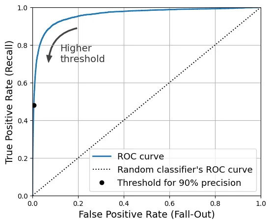
AUC (Area Under the Curve): Diện tích dưới đường cong ROC. AUC = 1 là hoàn hảo, AUC = 0.5 là ngẫu nhiên.
from sklearn.metrics import roc_auc_score

roc_auc_score(y_train_5, y_scores)
output:
0.9604938554008616So sánh với Random Forest Classifier:
Lưu ý: Random Forest không có decision_function, thay vào đó ta dùng predict_proba để lấy xác suất thuộc về lớp dương tính.
from sklearn.ensemble import RandomForestClassifier

forest_clf = RandomForestClassifier(random_state=42)

# RandomForest không có decision_function mà dùng predict_proba
y_probas_forest = cross_val_predict(forest_clf, X_train, y_train_5, cv=3,
method="predict_proba")y_probas_forest[:2]output:
array([[0.11, 0.89],
[0.99, 0.01]])Kiểm tra tính chính chuẩn của xác suất (Calibration):
# Not in the code - kiểm chứng xác suất ước lượng
idx_50_to_60 = (y_probas_forest[:, 1] > 0.50) & (y_probas_forest[:, 1] < 0.60)
print(f"{(y_train_5[idx_50_to_60]).sum() / idx_50_to_60.sum():.1%}")
output:
94.0%So sánh đường cong ROC giữa SGD và Random Forest.
y_scores_forest = y_probas_forest[:, 1]
precisions_forest, recalls_forest, thresholds_forest = precision_recall_curve(
    y_train_5, y_scores_forest)

plt.figure(figsize=(6, 5))  # extra code
plt.plot(recalls_forest, precisions_forest, "b-", linewidth=2,
         label="Random Forest")
plt.plot(recalls, precisions, "--", linewidth=2, label="SGD")

# extra code – trang trí cho Hình 3–8
plt.xlabel("Recall")
plt.ylabel("Precision")
plt.axis([0, 1, 0, 1])
plt.grid()
plt.legend(loc="lower left")
plt.show()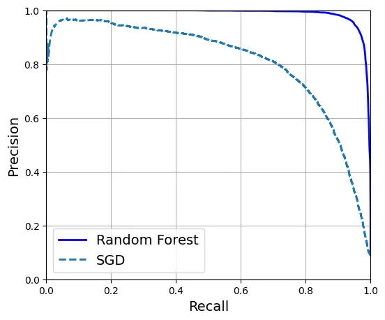
Random Forest vượt trội hơn hẳn với AUC gần bằng 1 và F1 score cao.
y_train_pred_forest = y_probas_forest[:, 1] >= 0.5  # xác suất >= 50% thì coi là dương tính
f1_score(y_train_5, y_train_pred_forest)
output:
0.9274509803921569roc_auc_score(y_train_5, y_scores_forest)output:
0.9983436731328145precision_score(y_train_5, y_train_pred_forest)output:
0.9897468089558485recall_score(y_train_5, y_train_pred_forest)output:
0.8725327430363402Phân loại Đa lớp (Multiclass Classification)
Bài toán bây giờ là phân biệt 10 chữ số (0-9). Có hai chiến lược chính để dùng bộ phân loại nhị phân cho đa lớp:
- OvR (One-versus-the-Rest): Huấn luyện 10 bộ phân loại, mỗi bộ phân biệt một số với tất cả các số còn lại. Chọn lớp có điểm số cao nhất.
- OvO (One-versus-One): Huấn luyện bộ phân loại cho từng cặp số (ví dụ: 0 vs 1, 0 vs 2…). Cần bộ phân loại.
SVM (Support Vector Machine) mở rộng không tốt với kích thước dữ liệu lớn (độ phức tạp huấn luyện khoảng đến ). Do đó, Scikit-Learn mặc định dùng OvO cho SVM để huấn luyện trên các tập con nhỏ hơn.
from sklearn.svm import SVC

svm_clf = SVC(random_state=42)
svm_clf.fit(X_train[:2000], y_train[:2000])  # Dùng y_train (nhãn gốc 0-9), không phải y_train_5
output:
SVC(random_state=42)Dự đoán:
svm_clf.predict([some_digit])output:
array(['5'], dtype=object)Điểm quyết định cho 10 lớp (do cơ chế voting của OvO):
some_digit_scores = svm_clf.decision_function([some_digit])
some_digit_scores.round(2)
output:
array([[ 3.79, 0.73, 6.06, 8.3 , -0.29, 9.3 , 1.75, 2.77, 7.21,
4.82]])class_id = some_digit_scores.argmax() # Tìm vị trí có điểm cao nhất
class_idoutput:
5svm_clf.classes_output:
array(['0', '1', '2', '3', '4', '5', '6', '7', '8', '9'], dtype=object)svm_clf.classes_[class_id]output:
'5'Nếu ép buộc dùng OvO, ta sẽ thấy 45 điểm số tương ứng với 45 cặp đấu ().
# extra code – hiển thị 45 điểm số cho 45 cặp đấu (10 chọn 2)
svm_clf.decision_function_shape = "ovo"
some_digit_scores_ovo = svm_clf.decision_function([some_digit])
some_digit_scores_ovo.round(2)
output:
array([[ 0.11, -0.21, -0.97, 0.51, -1.01, 0.19, 0.09, -0.31, -0.04,
-0.45, -1.28, 0.25, -1.01, -0.13, -0.32, -0.9 , -0.36, -0.93,
0.79, -1. , 0.45, 0.24, -0.24, 0.25, 1.54, -0.77, 1.11,
1.13, 1.04, 1.2 , -1.42, -0.53, -0.45, -0.99, -0.95, 1.21,
1. , 1. , 1.08, -0.02, -0.67, -0.14, -0.3 , -0.13, 0.25]])Sử dụng OneVsRestClassifier để ép buộc chiến lược OvR:
from sklearn.multiclass import OneVsRestClassifier

ovr_clf = OneVsRestClassifier(SVC(random_state=42))
ovr_clf.fit(X_train[:2000], y_train[:2000])
output:
OneVsRestClassifier(estimator=SVC(random_state=42))ovr_clf.predict([some_digit])output:
array(['5'], dtype='<U1')len(ovr_clf.estimators_) # Kiểm tra xem có đúng là 10 mô hình con khôngoutput:
10Với SGDClassifier, thuật toán này tự nhiên hỗ trợ xử lý dữ liệu lớn, nên Scikit-Learn mặc định dùng OvR.
sgd_clf = SGDClassifier(random_state=42)
sgd_clf.fit(X_train, y_train)
sgd_clf.predict([some_digit])
output:
array(['3'], dtype='<U1')Lưu ý: Ở đây SGD dự đoán sai là ‘3’. Điều này có thể xảy ra. Hãy xem điểm số quyết định.
sgd_clf.decision_function([some_digit]).round()output:
array([[-31893., -34420., -9531., 1824., -22320., -1386., -26189.,
-16148., -4604., -12051.]])Đánh giá mô hình SGD trên toàn bộ tập huấn luyện:
cross_val_score(sgd_clf, X_train, y_train, cv=3, scoring="accuracy")output:
array([0.87365, 0.85835, 0.8689 ])Kết quả khoảng 87%. Chúng ta có thể cải thiện bằng cách chuẩn hóa dữ liệu (Standard Scaling). Với SGD, việc các đặc trưng có cùng quy mô (scale) là cực kỳ quan trọng để Gradient Descent hội tụ nhanh và đúng hướng.
from sklearn.preprocessing import StandardScaler

scaler = StandardScaler()
X_train_scaled = scaler.fit_transform(X_train.astype("float64"))
cross_val_score(sgd_clf, X_train_scaled, y_train, cv=3, scoring="accuracy")
output:
array([0.8983, 0.891 , 0.9018])Độ chính xác tăng lên gần 90% chỉ nhờ vào việc chuẩn hóa.
Phân tích Lỗi (Error Analysis)
Chúng ta sử dụng Ma trận nhầm lẫn để xem mô hình hay nhầm lẫn giữa các số nào.
from sklearn.metrics import ConfusionMatrixDisplay

y_train_pred = cross_val_predict(sgd_clf, X_train_scaled, y_train, cv=3)
plt.rc('font', size=9)  # extra code – chỉnh font nhỏ lại cho vừa
ConfusionMatrixDisplay.from_predictions(y_train, y_train_pred)
plt.show()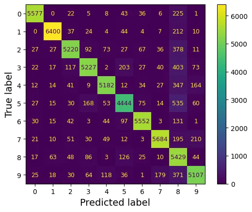
Chuẩn hóa ma trận theo hàng (True label) để so sánh tỷ lệ lỗi thay vì số lượng tuyệt đối.
plt.rc('font', size=10)  # extra code
ConfusionMatrixDisplay.from_predictions(y_train, y_train_pred,
                                        normalize="true", values_format=".0%")
plt.show()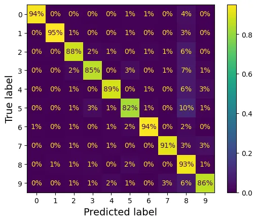
Để làm nổi bật các lỗi, ta xóa đường chéo chính (nơi dự đoán đúng).
sample_weight = (y_train_pred != y_train)
plt.rc('font', size=10)  # extra code
ConfusionMatrixDisplay.from_predictions(y_train, y_train_pred,
                                        sample_weight=sample_weight,
                                        normalize="true", values_format=".0%")
plt.show()
Trực quan hóa so sánh:
# extra code – tạo Hình 3–9
fig, axs = plt.subplots(nrows=1, ncols=2, figsize=(9, 4))
plt.rc('font', size=9)
ConfusionMatrixDisplay.from_predictions(y_train, y_train_pred, ax=axs[0])
axs[0].set_title("Confusion matrix")
plt.rc('font', size=10)
ConfusionMatrixDisplay.from_predictions(y_train, y_train_pred, ax=axs[1],
                                        normalize="true", values_format=".0%")
axs[1].set_title("CM normalized by row")
plt.show()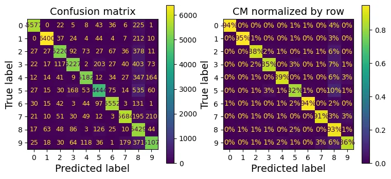
# extra code – tạo Hình 3–10
fig, axs = plt.subplots(nrows=1, ncols=2, figsize=(9, 4))
plt.rc('font', size=10)
ConfusionMatrixDisplay.from_predictions(y_train, y_train_pred, ax=axs[0],
                                        sample_weight=sample_weight,
                                        normalize="true", values_format=".0%")
axs[0].set_title("Errors normalized by row")
ConfusionMatrixDisplay.from_predictions(y_train, y_train_pred, ax=axs[1],
                                        sample_weight=sample_weight,
                                        normalize="pred", values_format=".0%")
axs[1].set_title("Errors normalized by column")
plt.show()
plt.rc('font', size=14)  # trả lại font chữ lớn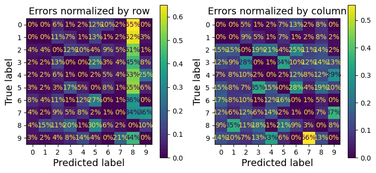
Phân tích sâu hơn các lỗi cụ thể, ví dụ cặp số 3 và 5. Đây là hai số có nét viết khá giống nhau.
cl_a, cl_b = '3', '5'
X_aa = X_train[(y_train == cl_a) & (y_train_pred == cl_a)] # 3 đoán là 3
X_ab = X_train[(y_train == cl_a) & (y_train_pred == cl_b)] # 3 đoán là 5 (Lỗi)
X_ba = X_train[(y_train == cl_b) & (y_train_pred == cl_a)] # 5 đoán là 3 (Lỗi)
X_bb = X_train[(y_train == cl_b) & (y_train_pred == cl_b)] # 5 đoán là 5

# extra code – tạo Hình 3–11
size = 5
pad = 0.2
plt.figure(figsize=(size, size))
for images, (label_col, label_row) in [(X_ba, (0, 0)), (X_bb, (1, 0)),
                                       (X_aa, (0, 1)), (X_ab, (1, 1))]:
    for idx, image_data in enumerate(images[:size*size]):
        x = idx % size + label_col * (size + pad)
        y = idx // size + label_row * (size + pad)
        plt.imshow(image_data.reshape(28, 28), cmap="binary",
                   extent=(x, x + 1, y, y + 1))
plt.xticks([size / 2, size + pad + size / 2], [str(cl_a), str(cl_b)])
plt.yticks([size / 2, size + pad + size / 2], [str(cl_b), str(cl_a)])
plt.plot([size + pad / 2, size + pad / 2], [0, 2 * size + pad], "k:")
plt.plot([0, 2 * size + pad], [size + pad / 2, size + pad / 2], "k:")
plt.axis([0, 2 * size + pad, 0, 2 * size + pad])
plt.xlabel("Predicted label")
plt.ylabel("True label")
plt.show()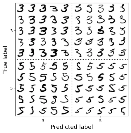
Phân loại Đa nhãn (Multilabel Classification)
Trong bài toán đa nhãn, đầu ra cho mỗi mẫu là một vector nhị phân , trong đó mỗi thể hiện sự hiện diện của một thuộc tính.
Ví dụ: Dự đoán (1) Số lớn () và (2) Số lẻ.
import numpy as np
from sklearn.neighbors import KNeighborsClassifier

y_train_large = (y_train >= '7')
y_train_odd = (y_train.astype('int8') % 2 == 1)
y_multilabel = np.c_[y_train_large, y_train_odd] # Kết hợp 2 nhãn lại

knn_clf = KNeighborsClassifier()
knn_clf.fit(X_train, y_multilabel)
output:
KNeighborsClassifier()Dự đoán cho số 5: Không lớn hơn 7 (False), là số lẻ (True).
knn_clf.predict([some_digit])output:
array([[False, True]])Đánh giá bằng F1 Score trung bình (macro average):
y_train_knn_pred = cross_val_predict(knn_clf, X_train, y_multilabel, cv=3)
f1_score(y_multilabel, y_train_knn_pred, average="macro")
output:
0.9764102655606048Nếu các nhãn không cân bằng, ta dùng average="weighted" để gán trọng số theo số lượng mẫu của mỗi nhãn.
# extra code – kiểm tra average="weighted"
f1_score(y_multilabel, y_train_knn_pred, average="weighted")
output:
0.9778357403921755Với các bộ phân loại không hỗ trợ đa nhãn tự nhiên (như SVM), ta dùng ClassifierChain.
from sklearn.multioutput import ClassifierChain

chain_clf = ClassifierChain(SVC(), cv=3, random_state=42)
chain_clf.fit(X_train[:2000], y_multilabel[:2000])
output:
ClassifierChain(base_estimator=SVC(), cv=3, random_state=42)chain_clf.predict([some_digit])output:
array([[0., 1.]])Phân loại Đa đầu ra (Multioutput Classification)
Đây là trường hợp tổng quát nhất, mỗi nhãn có thể nhận nhiều giá trị (không chỉ 0/1). Ví dụ: Khử nhiễu ảnh. Đầu ra là 784 pixel, mỗi pixel có giá trị từ 0 đến 255.
rng = np.random.default_rng(seed=42)
noise_train = rng.integers(0, 100, (len(X_train), 784)) # Tạo nhiễu ngẫu nhiên
X_train_mod = X_train + noise_train
noise_test = rng.integers(0, 100, (len(X_test), 784))
X_test_mod = X_test + noise_test
y_train_mod = X_train
y_test_mod = X_test

# extra code – tạo Hình 3–12
plt.subplot(121); plot_digit(X_test_mod[0])
plt.subplot(122); plot_digit(y_test_mod[0])
plt.show()
knn_clf = KNeighborsClassifier()
knn_clf.fit(X_train_mod, y_train_mod)
clean_digit = knn_clf.predict([X_test_mod[0]])
plot_digit(clean_digit)
plt.show()
Phần mở rộng
1. Bộ phân loại MNIST với độ chính xác trên 97%
Mục tiêu: Đạt độ chính xác > 97% trên tập test MNIST.
Chúng ta sẽ sử dụng KNN và tinh chỉnh siêu tham số weights (trọng số khoảng cách) và n_neighbors (số láng giềng).
Baseline (Mặc định):
knn_clf = KNeighborsClassifier()
knn_clf.fit(X_train, y_train)
baseline_accuracy = knn_clf.score(X_test, y_test)
baseline_accuracy
output:
0.9688Sử dụng GridSearchCV để tìm tham số tối ưu.
from sklearn.model_selection import GridSearchCV

param_grid = [{'weights': ["uniform", "distance"], 'n_neighbors': [3, 4, 5, 6]}]
knn_clf = KNeighborsClassifier()
grid_search = GridSearchCV(knn_clf, param_grid, cv=5)
grid_search.fit(X_train[:10_000], y_train[:10_000])
output:
GridSearchCV(cv=5, estimator=KNeighborsClassifier(),
param_grid=[{'n_neighbors': [3, 4, 5, 6],
'weights': ['uniform', 'distance']}])grid_search.best_params_output:
{'n_neighbors': 4, 'weights': 'distance'}grid_search.best_score_output:
0.9441999999999998Huấn luyện lại trên toàn bộ tập dữ liệu với tham số tốt nhất:
grid_search.best_estimator_.fit(X_train, y_train)
tuned_accuracy = grid_search.score(X_test, y_test)
tuned_accuracy
output:
0.9714Đạt 97.14%. Thành công!
2. Tăng cường dữ liệu (Data Augmentation)
Kỹ thuật này mở rộng tập huấn luyện bằng cách tạo ra các biến thể nhân tạo của dữ liệu gốc (dịch chuyển ảnh). Điều này giúp mô hình học được tính bất biến (invariance) đối với vị trí.
from scipy.ndimage import shift

def shift_image(image, dx, dy):
    image = image.reshape((28, 28))
    # Dịch chuyển ảnh và lấp đầy khoảng trống bằng 0 (màu trắng/đen tùy nền)
    shifted_image = shift(image, [dy, dx], cval=0, mode="constant")
    return shifted_image.reshape([-1])
image = X_train[1000] # lấy một chữ số ngẫu nhiên
shifted_image_down = shift_image(image, 0, 5)
shifted_image_left = shift_image(image, -5, 0)
plt.figure(figsize=(12, 3))
plt.subplot(131)
plt.title("Original")
plt.imshow(image.reshape(28, 28),
interpolation="nearest", cmap="Greys")
plt.subplot(132)
plt.title("Shifted down")
plt.imshow(shifted_image_down.reshape(28, 28),
interpolation="nearest", cmap="Greys")
plt.subplot(133)
plt.title("Shifted left")
plt.imshow(shifted_image_left.reshape(28, 28),
interpolation="nearest", cmap="Greys")
plt.show()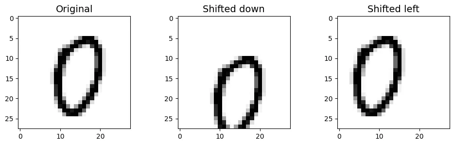
Tạo dữ liệu mở rộng:
X_train_augmented = [image for image in X_train]
y_train_augmented = [label for label in y_train]

for dx, dy in ((-1, 0), (1, 0), (0, 1), (0, -1)): # 4 hướng
    for image, label in zip(X_train, y_train):
        X_train_augmented.append(shift_image(image, dx, dy))
        y_train_augmented.append(label)

X_train_augmented = np.array(X_train_augmented)
y_train_augmented = np.array(y_train_augmented)
Xáo trộn dữ liệu (Shuffle) là bước quan trọng để phá vỡ thứ tự của các mẫu nhân tạo.
rng = np.random.default_rng(seed=42)
shuffle_idx = rng.permutation(len(X_train_augmented))
X_train_augmented = X_train_augmented[shuffle_idx]
y_train_augmented = y_train_augmented[shuffle_idx]
Huấn luyện mô hình KNN tối ưu trên tập dữ liệu lớn hơn này.
knn_clf = KNeighborsClassifier(**grid_search.best_params_)
knn_clf.fit(X_train_augmented, y_train_augmented)
output:
KNeighborsClassifier(n_neighbors=4, weights='distance')augmented_accuracy = knn_clf.score(X_test, y_test)
augmented_accuracyoutput:
0.9763Hiệu suất tăng lên 97.63%. Việc giảm tỷ lệ lỗi (error rate) là đáng kể.
error_rate_change = (1 - augmented_accuracy) / (1 - tuned_accuracy) - 1
print(f"error_rate_change = {error_rate_change:.0%}")
output:
error_rate_change = -17%3. Thử thách với bộ dữ liệu Titanic
Dự đoán khả năng sống sót trên tàu Titanic. Đây là bài toán kết hợp dữ liệu số, phân loại và xử lý dữ liệu thiếu.
from pathlib import Path
import pandas as pd
import tarfile
import urllib.request

def load_titanic_data():
    tarball_path = Path("datasets/titanic.tgz")
    if not tarball_path.is_file():
        Path("datasets").mkdir(parents=True, exist_ok=True)
        url = "https://github.com/ageron/data/raw/main/titanic.tgz"
        urllib.request.urlretrieve(url, tarball_path)
        with tarfile.open(tarball_path) as titanic_tarball:
            titanic_tarball.extractall(path="datasets", filter="data")
    return [pd.read_csv(Path("datasets/titanic") / filename)
            for filename in ("train.csv", "test.csv")]

train_data, test_data = load_titanic_data()train_data.head()output:
PassengerId Survived Pclass \
0 1 0 3
1 2 1 1
2 3 1 3
3 4 1 1
4 5 0 3
Name Sex Age SibSp \
0 Braund, Mr. Owen Harris male 22.0 1
1 Cumings, Mrs. John Bradley (Florence Briggs Th... female 38.0 1
2 Heikkinen, Miss. Laina female 26.0 0
3 Futrelle, Mrs. Jacques Heath (Lily May Peel) female 35.0 1
4 Allen, Mr. William Henry male 35.0 0
Parch Ticket Fare Cabin Embarked
0 0 A/5 21171 7.2500 NaN S
1 0 PC 17599 71.2833 C85 C
2 0 STON/O2. 3101282 7.9250 NaN S
3 0 113803 53.1000 C123 S
4 0 373450 8.0500 NaN S train_data = train_data.set_index("PassengerId")
test_data = test_data.set_index("PassengerId")Phân tích dữ liệu thiếu:
train_data.info()output:
<class 'pandas.core.frame.DataFrame'>
Index: 891 entries, 1 to 891
Data columns (total 11 columns):
# Column Non-Null Count Dtype
--- ------ -------------- -----
0 Survived 891 non-null int64
1 Pclass 891 non-null int64
2 Name 891 non-null object
3 Sex 891 non-null object
4 Age 714 non-null float64
5 SibSp 891 non-null int64
6 Parch 891 non-null int64
7 Ticket 891 non-null object
8 Fare 891 non-null float64
9 Cabin 204 non-null object
10 Embarked 889 non-null object
dtypes: float64(2), int64(4), object(5)
memory usage: 83.5+ KBtrain_data[train_data["Sex"]=="female"]["Age"].median()output:
27.0train_data.describe()output:
Survived Pclass Age SibSp Parch Fare
count 891.000000 891.000000 714.000000 891.000000 891.000000 891.000000
mean 0.383838 2.308642 29.699113 0.523008 0.381594 32.204208
std 0.486592 0.836071 14.526507 1.102743 0.806057 49.693429
min 0.000000 1.000000 0.416700 0.000000 0.000000 0.000000
25% 0.000000 2.000000 20.125000 0.000000 0.000000 7.910400
50% 0.000000 3.000000 28.000000 0.000000 0.000000 14.454200
75% 1.000000 3.000000 38.000000 1.000000 0.000000 31.000000
max 1.000000 3.000000 80.000000 8.000000 6.000000 512.329200train_data["Survived"].value_counts()output:
Survived
0 549
1 342
Name: count, dtype: int64train_data["Pclass"].value_counts()output:
Pclass
3 491
1 216
2 184
Name: count, dtype: int64train_data["Sex"].value_counts()output:
Sex
male 577
female 314
Name: count, dtype: int64train_data["Embarked"].value_counts()output:
Embarked
S 644
C 168
Q 77
Name: count, dtype: int64Pipeline xử lý:
- Dữ liệu số (Numerical): Điền giá trị thiếu bằng Median, sau đó chuẩn hóa (StandardScaler).
- Dữ liệu phân loại (Categorical): Điền giá trị thiếu bằng Most Frequent, sau đó mã hóa OneHot.
from sklearn.pipeline import Pipeline
from sklearn.impute import SimpleImputer
from sklearn.preprocessing import StandardScaler

num_pipeline = Pipeline([
        ("imputer", SimpleImputer(strategy="median")),
        ("scaler", StandardScaler())
    ])
from sklearn.preprocessing import OrdinalEncoder, OneHotEncoder
cat_pipeline = Pipeline([
("ordinal_encoder", OrdinalEncoder()),
("imputer", SimpleImputer(strategy="most_frequent")),
("cat_encoder", OneHotEncoder(sparse_output=False)),
])from sklearn.compose import ColumnTransformer
num_attribs = ["Age", "SibSp", "Parch", "Fare"]
cat_attribs = ["Pclass", "Sex", "Embarked"]
preprocess_pipeline = ColumnTransformer([
("num", num_pipeline, num_attribs),
("cat", cat_pipeline, cat_attribs),
])X_train = preprocess_pipeline.fit_transform(train_data)
X_trainoutput:
array([[-0.56573582, 0.43279337, -0.47367361, ..., 0. ,
0. , 1. ],
[ 0.6638609 , 0.43279337, -0.47367361, ..., 1. ,
0. , 0. ],
[-0.25833664, -0.4745452 , -0.47367361, ..., 0. ,
0. , 1. ],
...,
[-0.10463705, 0.43279337, 2.00893337, ..., 0. ,
0. , 1. ],
[-0.25833664, -0.4745452 , -0.47367361, ..., 1. ,
0. , 0. ],
[ 0.20276213, -0.4745452 , -0.47367361, ..., 0. ,
1. , 0. ]])y_train = train_data["Survived"]Huấn luyện mô hình Random Forest:
forest_clf = RandomForestClassifier(n_estimators=100, random_state=42)
forest_clf.fit(X_train, y_train)
output:
RandomForestClassifier(random_state=42)Dự đoán và đánh giá:
X_test = preprocess_pipeline.transform(test_data)
y_pred = forest_clf.predict(X_test)
forest_scores = cross_val_score(forest_clf, X_train, y_train, cv=10)
forest_scores.mean()output:
0.8137578027465668So sánh với SVM:
from sklearn.svm import SVC

svm_clf = SVC(gamma="auto")
svm_scores = cross_val_score(svm_clf, X_train, y_train, cv=10)
svm_scores.mean()
output:
0.8249313358302123Vẽ biểu đồ hộp (Box Plot) để so sánh phân phối độ chính xác giữa hai mô hình qua 10 folds.
plt.figure(figsize=(8, 4))
plt.plot([1]*10, svm_scores, ".")
plt.plot([2]*10, forest_scores, ".")
plt.boxplot([svm_scores, forest_scores], labels=("SVM", "Random Forest"))
plt.ylabel("Accuracy")
plt.show()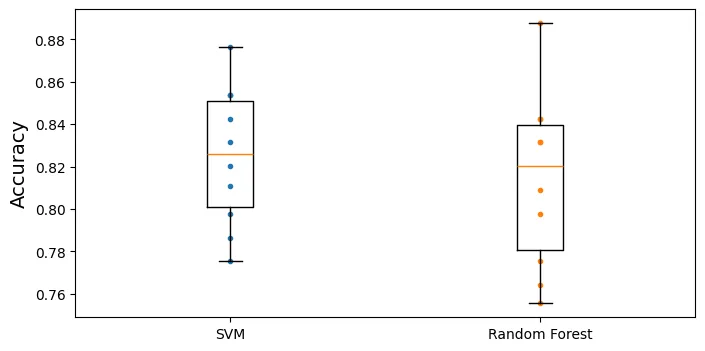
Kỹ thuật Feature Engineering (Tạo đặc trưng mới):
train_data["AgeBucket"] = train_data["Age"] // 15 * 15
train_data[["AgeBucket", "Survived"]].groupby(['AgeBucket']).mean()
output:
Survived
AgeBucket
0.0 0.576923
15.0 0.362745
30.0 0.423256
45.0 0.404494
60.0 0.240000
75.0 1.000000train_data["RelativesOnboard"] = train_data["SibSp"] + train_data["Parch"]
train_data[["RelativesOnboard", "Survived"]].groupby(
['RelativesOnboard']).mean()output:
Survived
RelativesOnboard
0 0.303538
1 0.552795
2 0.578431
3 0.724138
4 0.200000
5 0.136364
6 0.333333
7 0.000000
10 0.0000004. Bộ phân loại Spam (Spam Classifier)
Bài toán Xử lý Ngôn ngữ Tự nhiên (NLP) điển hình. Mục tiêu là phân loại email thành Ham (thư thường) và Spam (thư rác).
import tarfile

def fetch_spam_data():
    spam_root = "http://spamassassin.apache.org/old/publiccorpus/"
    ham_url = spam_root + "20030228_easy_ham.tar.bz2"
    spam_url = spam_root + "20030228_spam.tar.bz2"

    spam_path = Path() / "datasets" / "spam"
    spam_path.mkdir(parents=True, exist_ok=True)
    for dir_name, tar_name, url in (("easy_ham", "ham", ham_url),
                                    ("spam", "spam", spam_url)):
        if not (spam_path / dir_name).is_dir():
            path = (spam_path / tar_name).with_suffix(".tar.bz2")
            print("Downloading", path)
            urllib.request.urlretrieve(url, path)
            tar_bz2_file = tarfile.open(path)
            tar_bz2_file.extractall(path=spam_path, filter="data")
            tar_bz2_file.close()
    return [spam_path / dir_name for dir_name in ("easy_ham", "spam")]

ham_dir, spam_dir = fetch_spam_data()
output:
Downloading datasets/spam/ham.tar.bz2
Downloading datasets/spam/spam.tar.bz2ham_filenames = [f for f in sorted(ham_dir.iterdir()) if len(f.name) > 20]
spam_filenames = [f for f in sorted(spam_dir.iterdir()) if len(f.name) > 20]
len(ham_filenames)output:
2500len(spam_filenames)output:
500Phân tích (Parse) email:
import email
import email.policy

def load_email(filepath):
    with open(filepath, "rb") as f:
        return email.parser.BytesParser(policy=email.policy.default).parse(f)

ham_emails = [load_email(filepath) for filepath in ham_filenames]
spam_emails = [load_email(filepath) for filepath in spam_filenames]print(ham_emails[1].get_content().strip())output:
Martin A posted:
Tassos Papadopoulos, the Greek sculptor behind the plan, judged that the
limestone of Mount Kerdylio, 70 miles east of Salonika and not far from the
Mount Athos monastic community, was ideal for the patriotic sculpture.
As well as Alexander's granite features, 240 ft high and 170 ft wide, a
museum, a restored amphitheatre and car park for admiring crowds are
planned
---------------------
So is this mountain limestone or granite?
If it's limestone, it'll weather pretty fast.
------------------------ Yahoo! Groups Sponsor ---------------------~-->
4 DVDs Free +s&p Join Now
http://us.click.yahoo.com/pt6YBB/NXiEAA/mG3HAA/7gSolB/TM
---------------------------------------------------------------------~->
To unsubscribe from this group, send an email to:
forteana-unsubscribe@egroups.com
Your use of Yahoo! Groups is subject to http://docs.yahoo.com/info/terms/print(spam_emails[6].get_content().strip())output:
Help wanted. We are a 14 year old fortune 500 company, that is
growing at a tremendous rate. We are looking for individuals who
want to work from home.
This is an opportunity to make an excellent income. No experience
is required. We will train you.
So if you are looking to be employed from home with a career that has
vast opportunities, then go:
http://www.basetel.com/wealthnow
We are looking for energetic and self motivated people. If that is you
than click on the link and fill out the form, and one of our
employement specialist will contact you.
To be removed from our link simple go to:
http://www.basetel.com/remove.html
4139vOLW7-758DoDY1425FRhM1-764SMFc8513fCsLl40Xử lý cấu trúc đa phần (Multipart) của email:
def get_email_structure(email):
    if isinstance(email, str):
        return email
    payload = email.get_payload()
    if isinstance(payload, list):
        multipart = ", ".join([get_email_structure(sub_email)
                               for sub_email in payload])
        return f"multipart({multipart})"
    else:
        return email.get_content_type()

from collections import Counter

def structures_counter(emails):
    structures = Counter()
    for email in emails:
        structure = get_email_structure(email)
        structures[structure] += 1
return structuresstructures_counter(ham_emails).most_common()output:
[('text/plain', 2408),
('multipart(text/plain, application/pgp-signature)', 66),
('multipart(text/plain, text/html)', 8),
('multipart(text/plain, text/plain)', 4),
('multipart(text/plain)', 3),
('multipart(text/plain, application/octet-stream)', 2),
('multipart(text/plain, text/enriched)', 1),
('multipart(text/plain, application/ms-tnef, text/plain)', 1),
('multipart(multipart(text/plain, text/plain, text/plain), application/pgp-signature)',
1),
('multipart(text/plain, video/mng)', 1),
('multipart(text/plain, multipart(text/plain))', 1),
('multipart(text/plain, application/x-pkcs7-signature)', 1),
('multipart(text/plain, multipart(text/plain, text/plain), text/rfc822-headers)',
1),
('multipart(text/plain, multipart(text/plain, text/plain), multipart(multipart(text/plain, application/x-pkcs7-signature)))',
1),
('multipart(text/plain, application/x-java-applet)', 1)]structures_counter(spam_emails).most_common()output:
[('text/plain', 218),
('text/html', 183),
('multipart(text/plain, text/html)', 45),
('multipart(text/html)', 20),
('multipart(text/plain)', 19),
('multipart(multipart(text/html))', 5),
('multipart(text/plain, image/jpeg)', 3),
('multipart(text/html, application/octet-stream)', 2),
('multipart(text/plain, application/octet-stream)', 1),
('multipart(text/html, text/plain)', 1),
('multipart(multipart(text/html), application/octet-stream, image/jpeg)', 1),
('multipart(multipart(text/plain, text/html), image/gif)', 1),
('multipart/alternative', 1)]for header, value in spam_emails[0].items():
print(header, ":", value)output:
Return-Path : <12a1mailbot1@web.de>
Delivered-To : zzzz@localhost.spamassassin.taint.org
Received : from localhost (localhost [127.0.0.1]) by phobos.labs.spamassassin.taint.org (Postfix) with ESMTP id 136B943C32 for <zzzz@localhost>; Thu, 22 Aug 2002 08:17:21 -0400 (EDT)
Received : from mail.webnote.net [193.120.211.219] by localhost with POP3 (fetchmail-5.9.0) for zzzz@localhost (single-drop); Thu, 22 Aug 2002 13:17:21 +0100 (IST)
Received : from dd_it7 ([210.97.77.167]) by webnote.net (8.9.3/8.9.3) with ESMTP id NAA04623 for <zzzz@spamassassin.taint.org>; Thu, 22 Aug 2002 13:09:41 +0100
From : 12a1mailbot1@web.de
Received : from r-smtp.korea.com - 203.122.2.197 by dd_it7 with Microsoft SMTPSVC(5.5.1775.675.6); Sat, 24 Aug 2002 09:42:10 +0900
To : dcek1a1@netsgo.com
Subject : Life Insurance - Why Pay More?
Date : Wed, 21 Aug 2002 20:31:57 -1600
MIME-Version : 1.0
Message-ID : <0103c1042001882DD_IT7@dd_it7>
Content-Type : text/html; charset="iso-8859-1"
Content-Transfer-Encoding : quoted-printablespam_emails[0]["Subject"]output:
'Life Insurance - Why Pay More?'import numpy as np
from sklearn.model_selection import train_test_split
X = np.array(ham_emails + spam_emails, dtype=object)
y = np.array([0] * len(ham_emails) + [1] * len(spam_emails))
X_train, X_test, y_train, y_test = train_test_split(X, y, test_size=0.2,
random_state=42)Chuyển đổi HTML sang Plain Text:
import re
from html import unescape

def html_to_plain_text(html):
    text = re.sub(r'<head.*?>.*?</head>', '', html, flags=re.M | re.S | re.I)
    text = re.sub(r'<a\s.*?>', ' HYPERLINK ', text, flags=re.M | re.S | re.I)
    text = re.sub(r'<.*?>', '', text, flags=re.M | re.S)
    text = re.sub(r'(\s*\n)+', '\n', text, flags=re.M | re.S)
    return unescape(text)
html_spam_emails = [email for email in X_train[y_train==1]
if get_email_structure(email) == "text/html"]
sample_html_spam = html_spam_emails[7]
print(sample_html_spam.get_content().strip()[:1000], "...")output:
<HTML><HEAD><TITLE></TITLE><META http-equiv="Content-Type" content="text/html; charset=windows-1252"><STYLE>A:link {TEX-DECORATION: none}A:active {TEXT-DECORATION: none}A:visited {TEXT-DECORATION: none}A:hover {COLOR: #0033ff; TEXT-DECORATION: underline}</STYLE><META content="MSHTML 6.00.2713.1100" name="GENERATOR"></HEAD>
<BODY text="#000000" vLink="#0033ff" link="#0033ff" bgColor="#CCCC99"><TABLE borderColor="#660000" cellSpacing="0" cellPadding="0" border="0" width="100%"><TR><TD bgColor="#CCCC99" valign="top" colspan="2" height="27">
<font size="6" face="Arial, Helvetica, sans-serif" color="#660000">
<b>OTC</b></font></TD></TR><TR><TD height="2" bgcolor="#6a694f">
<font size="5" face="Times New Roman, Times, serif" color="#FFFFFF">
<b> Newsletter</b></font></TD><TD height="2" bgcolor="#6a694f"><div align="right"><font color="#FFFFFF">
<b>Discover Tomorrow's Winners </b></font></div></TD></TR><TR><TD height="25" colspan="2" bgcolor="#CCCC99"><table width="100%" border="0" ...print(html_to_plain_text(sample_html_spam.get_content())[:1000], "...")output:
OTC
Newsletter
Discover Tomorrow's Winners
For Immediate Release
Cal-Bay (Stock Symbol: CBYI)
Watch for analyst "Strong Buy Recommendations" and several advisory newsletters picking CBYI. CBYI has filed to be traded on the OTCBB, share prices historically INCREASE when companies get listed on this larger trading exchange. CBYI is trading around 25 cents and should skyrocket to $2.66 - $3.25 a share in the near future.
Put CBYI on your watch list, acquire a position TODAY.
REASONS TO INVEST IN CBYI
A profitable company and is on track to beat ALL earnings estimates!
One of the FASTEST growing distributors in environmental & safety equipment instruments.
Excellent management team, several EXCLUSIVE contracts. IMPRESSIVE client list including the U.S. Air Force, Anheuser-Busch, Chevron Refining and Mitsubishi Heavy Industries, GE-Energy & Environmental Research.
RAPIDLY GROWING INDUSTRY
Industry revenues exceed $900 million, estimates indicate that there could be as much as $25 billi ...def email_to_text(email):
html = None
for part in email.walk():
ctype = part.get_content_type()
if not ctype in ("text/plain", "text/html"):
continue
try:
content = part.get_content()
except: # phòng trường hợp lỗi encoding
content = str(part.get_payload())
if ctype == "text/plain":
return content
else:
html = content
if html:
return html_to_plain_text(html)
print(email_to_text(sample_html_spam)[:100], "...")output:
OTC
Newsletter
Discover Tomorrow's Winners
For Immediate Release
Cal-Bay (Stock Symbol: CBYI)
Wat ...Stemming với NLTK:
import nltk

stemmer = nltk.PorterStemmer()
for word in ("Computations", "Computation", "Computing", "Computed", "Compute",
             "Compulsive"):
    print(word, "=>", stemmer.stem(word))
output:
Computations => comput
Computation => comput
Computing => comput
Computed => comput
Compute => comput
Compulsive => compulsURL Extraction:
# Kiểm tra xem notebook đang chạy trên Colab hay Kaggle
IS_COLAB = "google.colab" in sys.modules
IS_KAGGLE = "kaggle_secrets" in sys.modules

# Nếu chạy trên Colab/Kaggle thì cài đặt urlextract
if IS_COLAB or IS_KAGGLE:
    %pip install -q -U urlextract
import urlextract # có thể yêu cầu kết nối mạng để tải danh sách domain
url_extractor = urlextract.URLExtract()
some_text = "Will it detect github.com and
print(url_extractor.find_urls(some_text))output:
['github.com', 'Biến đổi Email thành bộ đếm từ (Bag-of-Words):
from sklearn.base import BaseEstimator, TransformerMixin

class EmailToWordCounterTransformer(BaseEstimator, TransformerMixin):
    def __init__(self, strip_headers=True, lower_case=True,
                 remove_punctuation=True, replace_urls=True,
                 replace_numbers=True, stemming=True):
        self.strip_headers = strip_headers
        self.lower_case = lower_case
        self.remove_punctuation = remove_punctuation
        self.replace_urls = replace_urls
        self.replace_numbers = replace_numbers
        self.stemming = stemming
    def fit(self, X, y=None):
        return self
    def transform(self, X, y=None):
        X_transformed = []
        for email in X:
            text = email_to_text(email) or ""
            if self.lower_case:
                text = text.lower()
            if self.replace_urls and url_extractor is not None:
                urls = list(set(url_extractor.find_urls(text)))
                urls.sort(key=lambda url: len(url), reverse=True)
                for url in urls:
                    text = text.replace(url, " URL ")
            if self.replace_numbers:
                text = re.sub(r'\d+(?:\.\d*)?(?:[eE][+-]?\d+)?', 'NUMBER', text)
            if self.remove_punctuation:
                text = re.sub(r'\W+', ' ', text, flags=re.M)
            word_counts = Counter(text.split())
            if self.stemming and stemmer is not None:
                stemmed_word_counts = Counter()
                for word, count in word_counts.items():
                    stemmed_word = stemmer.stem(word)
                    stemmed_word_counts[stemmed_word] += count
                word_counts = stemmed_word_counts
            X_transformed.append(word_counts)
        return np.array(X_transformed)
X_few = X_train[:3]
X_few_wordcounts = EmailToWordCounterTransformer().fit_transform(X_few)
X_few_wordcountsoutput:
array([Counter({'chuck': 1, 'murcko': 1, 'wrote': 1, 'stuff': 1, 'yawn': 1, 'r': 1}),
Counter({'the': 11, 'of': 9, 'and': 8, 'all': 3, 'christian': 3, 'to': 3, 'by': 3, 'jefferson': 2, 'i': 2, 'have': 2, 'superstit': 2, 'one': 2, 'on': 2, 'been': 2, 'ha': 2, 'half': 2, 'rogueri': 2, 'teach': 2, 'jesu': 2, 'some': 1, 'interest': 1, 'quot': 1, 'url': 1, 'thoma': 1, 'examin': 1, 'known': 1, 'word': 1, 'do': 1, 'not': 1, 'find': 1, 'in': 1, 'our': 1, 'particular': 1, 'redeem': 1, 'featur': 1, 'they': 1, 'are': 1, 'alik': 1, 'found': 1, 'fabl': 1, 'mytholog': 1, 'million': 1, 'innoc': 1, 'men': 1, 'women': 1, 'children': 1, 'sinc': 1, 'introduct': 1, 'burnt': 1, 'tortur': 1, 'fine': 1, 'imprison': 1, 'what': 1, 'effect': 1, 'thi': 1, 'coercion': 1, 'make': 1, 'world': 1, 'fool': 1, 'other': 1, 'hypocrit': 1, 'support': 1, 'error': 1, 'over': 1, 'earth': 1, 'six': 1, 'histor': 1, 'american': 1, 'john': 1, 'e': 1, 'remsburg': 1, 'letter': 1, 'william': 1, 'short': 1, 'again': 1, 'becom': 1, 'most': 1, 'pervert': 1, 'system': 1, 'that': 1, 'ever': 1, 'shone': 1, 'man': 1, 'absurd': 1, 'untruth': 1, 'were': 1, 'perpetr': 1, 'upon': 1, 'a': 1, 'larg': 1, 'band': 1, 'dupe': 1, 'import': 1, 'led': 1, 'paul': 1, 'first': 1, 'great': 1, 'corrupt': 1}),
Counter({'url': 4, 's': 3, 'group': 3, 'to': 3, 'in': 2, 'forteana': 2, 'martin': 2, 'an': 2, 'and': 2, 'we': 2, 'is': 2, 'yahoo': 2, 'unsubscrib': 2, 'y': 1, 'adamson': 1, 'wrote': 1, 'for': 1, 'altern': 1, 'rather': 1, 'more': 1, 'factual': 1, 'base': 1, 'rundown': 1, 'on': 1, 'hamza': 1, 'career': 1, 'includ': 1, 'hi': 1, 'belief': 1, 'that': 1, 'all': 1, 'non': 1, 'muslim': 1, 'yemen': 1, 'should': 1, 'be': 1, 'murder': 1, 'outright': 1, 'know': 1, 'how': 1, 'unbias': 1, 'memri': 1, 'don': 1, 't': 1, 'html': 1, 'rob': 1, 'sponsor': 1, 'number': 1, 'dvd': 1, 'free': 1, 'p': 1, 'join': 1, 'now': 1, 'from': 1, 'thi': 1, 'send': 1, 'email': 1, 'egroup': 1, 'com': 1, 'your': 1, 'use': 1, 'of': 1, 'subject': 1})],
dtype=object)Chuyển đổi sang Vector số (Sparse Matrix):
from scipy.sparse import csr_matrix

class WordCounterToVectorTransformer(BaseEstimator, TransformerMixin):
    def __init__(self, vocabulary_size=1000):
        self.vocabulary_size = vocabulary_size
    def fit(self, X, y=None):
        total_count = Counter()
        for word_count in X:
            for word, count in word_count.items():
                total_count[word] += min(count, 10)
        most_common = total_count.most_common()[:self.vocabulary_size]
        self.vocabulary_ = {word: index + 1
                            for index, (word, count) in enumerate(most_common)}
        return self
    def transform(self, X, y=None):
        rows = []
        cols = []
        data = []
        for row, word_count in enumerate(X):
            for word, count in word_count.items():
                rows.append(row)
                cols.append(self.vocabulary_.get(word, 0))
                data.append(count)
        return csr_matrix((data, (rows, cols)),
                          shape=(len(X), self.vocabulary_size + 1))
vocab_transformer = WordCounterToVectorTransformer(vocabulary_size=10)
X_few_vectors = vocab_transformer.fit_transform(X_few_wordcounts)
X_few_vectorsoutput:
<Compressed Sparse Row sparse matrix of dtype 'int64'
with 20 stored elements and shape (3, 11)>X_few_vectors.toarray()output:
array([[ 6, 0, 0, 0, 0, 0, 0, 0, 0, 0, 0],
[99, 11, 9, 8, 3, 1, 3, 1, 3, 2, 3],
[67, 0, 1, 2, 3, 4, 1, 2, 0, 1, 0]])vocab_transformer.vocabulary_output:
{'the': 1,
'of': 2,
'and': 3,
'to': 4,
'url': 5,
'all': 6,
'in': 7,
'christian': 8,
'on': 9,
'by': 10}Huấn luyện LogisticRegression:
from sklearn.pipeline import Pipeline

preprocess_pipeline = Pipeline([
    ("email_to_wordcount", EmailToWordCounterTransformer()),
    ("wordcount_to_vector", WordCounterToVectorTransformer()),])

X_train_transformed = preprocess_pipeline.fit_transform(X_train)
from sklearn.linear_model import LogisticRegression
from sklearn.model_selection import cross_val_score
log_clf = LogisticRegression(max_iter=1000, random_state=42)
score = cross_val_score(log_clf, X_train_transformed, y_train, cv=3)
score.mean()output:
0.985from sklearn.metrics import precision_score, recall_score
X_test_transformed = preprocess_pipeline.transform(X_test)
log_clf = LogisticRegression(max_iter=1000, random_state=42)
log_clf.fit(X_train_transformed, y_train)
y_pred = log_clf.predict(X_test_transformed)
print(f"Precision: {precision_score(y_test, y_pred):.2%}")
print(f"Recall: {recall_score(y_test, y_pred):.2%}")output:
Precision: 96.88%
Recall: 97.89%