[ML101] Chương 2: Dự án Machine Learning đầu tiên
Hướng dẫn từng bước xây dựng dự án Machine Learning đầu tiên với Python
Bài viết có tham khảo, sử dụng và sửa đổi tài nguyên từ kho lưu trữ handson-mlp, tuân thủ giấy phép Apache‑2.0. Chúng tôi chân thành cảm ơn tác giả Aurélien Géron (@aureliengeron) vì sự chia sẻ kiến thức tuyệt vời và những đóng góp quý giá cho cộng đồng.
Chào mừng bạn đến với chương thực hành đầu tiên. Trong chương này, chúng ta sẽ đi qua toàn bộ quy trình của một dự án Machine Learning thực tế (End-to-End Machine Learning Project).
Mục tiêu của chúng ta là xây dựng một mô hình Hồi quy (Regression) – cụ thể là dự đoán giá nhà trung vị (median house value) tại các quận (districts) thuộc bang California. Mặc dù bạn đã đề cập đến bài toán phân loại, nhưng dựa trên bản chất dữ liệu (giá trị liên tục) và code, đây chính xác là một bài toán Hồi quy đa biến (Multivariate Regression). Chúng ta sẽ tiếp cận vấn đề này dưới góc độ toán học thống kê, từ việc xử lý dữ liệu thô, lựa chọn giả thuyết (hypothesis), tối ưu hàm mất mát (loss function) cho đến triển khai.
Bạn có thể chạy trực tiếp các đoạn mã code tại: Google Colab.
1. Thiết lập môi trường trên Google Colab
Để đảm bảo tính nhất quán và khả năng tái lập (reproducibility) của các thí nghiệm, việc kiểm soát phiên bản phần mềm là nên làm. Các thuật toán và API trong Machine Learning thay đổi thường xuyên; do đó, chúng ta cần xác nhận môi trường thực thi đáp ứng đúng yêu cầu.
Đoạn mã dưới đây kiểm tra phiên bản Python. Chúng ta yêu cầu Python 3.10+ để tận dụng các tính năng mới về type hinting và tối ưu hóa hiệu năng:
import sys

# Kiểm tra xem phiên bản Python có lớn hơn hoặc bằng 3.10 không
assert sys.version_info >= (3, 10)
Tiếp theo, chúng ta kiểm tra thư viện Scikit-Learn (sklearn). Đây là thư viện thông dụng cho các thuật toán Machine Learning cổ điển. Phiên bản 1.6.1 được yêu cầu để đảm bảo các hàm như LinearRegression hay KNeighborsRegressor hoạt động chính xác như trong Chương này.
from packaging.version import Version
import sklearn

# Kiểm tra phiên bản của thư viện Scikit-Learn
assert Version(sklearn.__version__) >= Version("1.6.1")
Chúng ta cũng thiết lập cấu hình cho Matplotlib để đảm bảo các biểu đồ hiển thị rõ ràng, hỗ trợ việc phân tích định lượng trên đồ thị.
import matplotlib.pyplot as plt

# Thiết lập kích thước phông chữ chung là 12
plt.rc('font', size=12)
# Thiết lập kích thước phông chữ cho nhãn trục (x, y) là 14
plt.rc('axes', labelsize=14, titlesize=14)
# Thiết lập kích thước phông chữ cho chú thích (legend) là 12
plt.rc('legend', fontsize=12)
# Thiết lập kích thước phông chữ cho các vạch chia trên trục x và y là 10
plt.rc('xtick', labelsize=10)
plt.rc('ytick', labelsize=10)
2. Thu thập Dữ liệu (Data Acquisition)
Dữ liệu là nhiên liệu của các mô hình học thống kê. Chúng ta sẽ làm việc với dữ liệu nhà ở California.
2.1. Tải dữ liệu
Đoạn mã dưới đây thiết lập một quy trình tự động hóa (automation pipeline) để tải và giải nén dữ liệu. Việc này giúp tách biệt mã nguồn khỏi dữ liệu cục bộ, cho phép luồng công việc hoạt động trên bất kỳ máy nào.
from pathlib import Path
import pandas as pd
import tarfile
import urllib.request

def load_housing_data():
    # Định nghĩa đường dẫn file nén
    tarball_path = Path("datasets/housing.tgz")

    # Nếu file chưa tồn tại, tiến hành tải về
    if not tarball_path.is_file():
        # Tạo thư mục datasets nếu chưa có
        Path("datasets").mkdir(parents=True, exist_ok=True)
        url = "https://github.com/ageron/data/raw/main/housing.tgz"
        # Tải file từ URL về đường dẫn local
        urllib.request.urlretrieve(url, tarball_path)

        # Giải nén file
        with tarfile.open(tarball_path) as housing_tarball:
            housing_tarball.extractall(path="datasets", filter="data")

    # Đọc file CSV vào Pandas DataFrame
    return pd.read_csv(Path("datasets/housing/housing.csv"))

# Gọi hàm để lấy dữ liệu
housing_full = load_housing_data()
2.2. Khám phá cấu trúc dữ liệu (Exploratory Data Analysis - EDA)
Trước khi áp dụng bất kỳ thuật toán nào, ta cần hiểu phân phối thống kê của dữ liệu.
housing_full.head()output:
longitude latitude housing_median_age total_rooms total_bedrooms \
0 -122.23 37.88 41.0 880.0 129.0
1 -122.22 37.86 21.0 7099.0 1106.0
2 -122.24 37.85 52.0 1467.0 190.0
3 -122.25 37.85 52.0 1274.0 235.0
4 -122.25 37.85 52.0 1627.0 280.0
population households median_income median_house_value ocean_proximity
0 322.0 126.0 8.3252 452600.0 NEAR BAY
1 2401.0 1138.0 8.3014 358500.0 NEAR BAY
2 496.0 177.0 7.2574 352100.0 NEAR BAY
3 558.0 219.0 5.6431 341300.0 NEAR BAY
4 565.0 259.0 3.8462 342200.0 NEAR BAY Phương thức info() cho ta cái nhìn tổng quan về kiểu dữ liệu và các giá trị bị thiếu (null). Lưu ý cột total_bedrooms chỉ có 20,433 giá trị so với 20,640 của tổng thể, tức là có dữ liệu bị khuyết. Đây là vấn đề cần xử lý trong bước tiền xử lý.
housing_full.info()output:
<class 'pandas.core.frame.DataFrame'>
RangeIndex: 20640 entries, 0 to 20639
Data columns (total 10 columns):
# Column Non-Null Count Dtype
--- ------ -------------- -----
0 longitude 20640 non-null float64
1 latitude 20640 non-null float64
2 housing_median_age 20640 non-null float64
3 total_rooms 20640 non-null float64
4 total_bedrooms 20433 non-null float64
5 population 20640 non-null float64
6 households 20640 non-null float64
7 median_income 20640 non-null float64
8 median_house_value 20640 non-null float64
9 ocean_proximity 20640 non-null object
dtypes: float64(9), object(1)
memory usage: 1.6+ MBPhân tích biến phân loại (categorical variable) ocean_proximity:
housing_full["ocean_proximity"].value_counts()output:
ocean_proximity
<1H OCEAN 9136
INLAND 6551
NEAR OCEAN 2658
NEAR BAY 2290
ISLAND 5
Name: count, dtype: int64Hàm describe() cung cấp các thống kê mô tả (descriptive statistics).
- std (Standard Deviation - ): Đo lường độ phân tán của dữ liệu.
- 25%, 50%, 75%: Các tứ phân vị (quartiles). 50% chính là trung vị (median).
housing_full.describe()output:
longitude latitude housing_median_age total_rooms \
count 20640.000000 20640.000000 20640.000000 20640.000000
mean -119.569704 35.631861 28.639486 2635.763081
std 2.003532 2.135952 12.585558 2181.615252
min -124.350000 32.540000 1.000000 2.000000
25% -121.800000 33.930000 18.000000 1447.750000
50% -118.490000 34.260000 29.000000 2127.000000
75% -118.010000 37.710000 37.000000 3148.000000
max -114.310000 41.950000 52.000000 39320.000000
total_bedrooms population households median_income \
count 20433.000000 20640.000000 20640.000000 20640.000000
mean 537.870553 1425.476744 499.539680 3.870671
std 421.385070 1132.462122 382.329753 1.899822
min 1.000000 3.000000 1.000000 0.499900
25% 296.000000 787.000000 280.000000 2.563400
50% 435.000000 1166.000000 409.000000 3.534800
75% 647.000000 1725.000000 605.000000 4.743250
max 6445.000000 35682.000000 6082.000000 15.000100
median_house_value
count 20640.000000
mean 206855.816909
std 115395.615874
min 14999.000000
25% 119600.000000
50% 179700.000000
75% 264725.000000
max 500001.000000 Biểu đồ Histogram giúp ta quan sát dạng phân phối xác suất (probability distribution). Quan sát output bên dưới:
- Các biến
housing_median_agevàmedian_house_valuebị giới hạn (capped). - Các biến này có phân phối đuôi dài (heavy-tailed), khác xa phân phối chuẩn (Gaussian). Điều này có thể gây khó khăn cho các thuật toán học máy.
import matplotlib.pyplot as plt

# extra code – các dòng sau thiết lập kích thước font chữ mặc định cho biểu đồ
plt.rc('font', size=14)
plt.rc('axes', labelsize=14, titlesize=14)
plt.rc('legend', fontsize=14)
plt.rc('xtick', labelsize=10)
plt.rc('ytick', labelsize=10)

# Vẽ histogram cho toàn bộ các cột số
housing_full.hist(bins=50, figsize=(12, 8))
plt.show()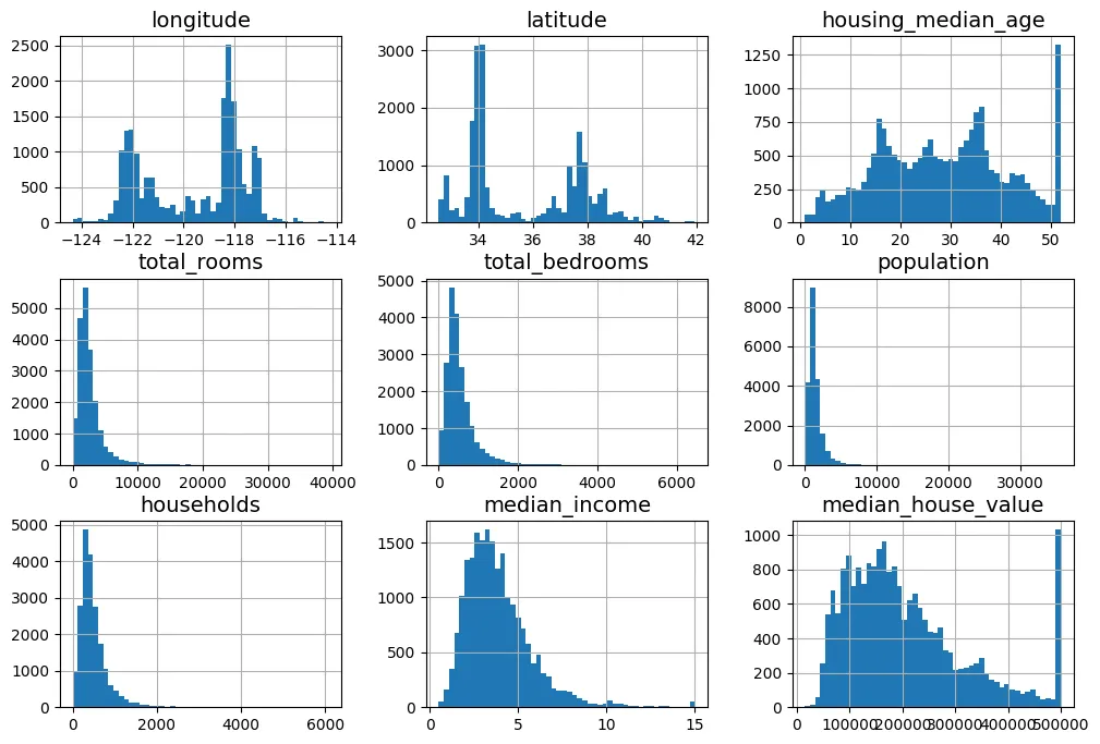
3. Tạo tập kiểm tra (Test Set)
Để đánh giá khách quan khả năng tổng quát hóa (generalization) của mô hình, chúng ta cần tách riêng một phần dữ liệu làm tập kiểm tra.
3.1. Lấy mẫu ngẫu nhiên (Random Sampling)
Chúng ta sử dụng một bộ sinh số ngẫu nhiên (RNG) để xáo trộn dữ liệu.
import numpy as np

def shuffle_and_split_data(data, test_ratio, rng):
    # Hoán vị ngẫu nhiên các chỉ số (index)
    shuffled_indices = rng.permutation(len(data))
    # Tính kích thước tập test
    test_set_size = int(len(data) * test_ratio)
    # Tách chỉ số cho test và train
    test_indices = shuffled_indices[:test_set_size]
    train_indices = shuffled_indices[test_set_size:]
    # Trả về 2 DataFrame tương ứng
    return data.iloc[train_indices], data.iloc[test_indices]
Việc đặt seed=42 là cực kỳ quan trọng để đảm bảo tính tất định (deterministic). Nó giúp kết quả chia tập dữ liệu giống hệt nhau mỗi lần chạy, phục vụ việc gỡ lỗi và so sánh.
# Tạo bộ sinh số ngẫu nhiên với seed cố định là 42
rng = np.random.default_rng(seed=42)
train_set, test_set = shuffle_and_split_data(housing_full, 0.2, rng)

# Kiểm tra kích thước tập train
len(train_set)
output:
16512# Kiểm tra kích thước tập test
len(test_set)output:
4128Để đảm bảo tính nhất quán ngay cả khi dữ liệu được cập nhật, ta có thể dùng kỹ thuật băm (hashing) định danh của mẫu dữ liệu.
from zlib import crc32

def is_id_in_test_set(identifier, test_ratio):
    # Kiểm tra xem mã hash của ID có nhỏ hơn ngưỡng tỉ lệ hay không
    return crc32(np.int64(identifier)) < test_ratio * 2**32

def split_data_with_id_hash(data, test_ratio, id_column):
    ids = data[id_column]
    # Áp dụng hàm kiểm tra cho từng ID
    in_test_set = ids.apply(lambda id_: is_id_in_test_set(id_, test_ratio))
    return data.loc[~in_test_set], data.loc[in_test_set]
Sử dụng index làm ID:
housing_with_id = housing_full.reset_index()  # thêm cột `index`
train_set, test_set = split_data_with_id_hash(housing_with_id, 0.2, "index")
Sử dụng tọa độ địa lý để tạo ID bất biến:
# Tạo ID từ kinh độ và vĩ độ
housing_with_id["id"] = (housing_full["longitude"] * 1000
                         + housing_full["latitude"])
train_set, test_set = split_data_with_id_hash(housing_with_id, 0.2, "id")
Tuy nhiên, Scikit-Learn cung cấp hàm train_test_split tối ưu hơn:
from sklearn.model_selection import train_test_split

train_set, test_set = train_test_split(housing_full, test_size=0.2,
                                       random_state=42)
Kiểm tra dữ liệu bị thiếu trong tập test:
test_set["total_bedrooms"].isnull().sum()output:
np.int64(44)3.2. Lấy mẫu phân tầng (Stratified Sampling)
Khi tập dữ liệu không đủ lớn, lấy mẫu ngẫu nhiên có thể dẫn đến sai lệch lấy mẫu (sampling bias). Để đảm bảo tập test đại diện đúng cho tổng thể, ta dùng phương pháp phân tầng. Giả sử median_income là yếu tố quan trọng nhất ảnh hưởng đến giá nhà, ta cần phân tầng theo biến này.
Đoạn mã dưới tính toán xác suất lý thuyết về việc lấy mẫu bị lệch:
# Đoạn mã mô phỏng xác suất (lý thuyết xác suất thống kê)
# extra code – tính xác suất mẫu xấu (10.7%)
from scipy.stats import binom

sample_size = 1000
ratio_female = 0.516
proba_too_small = binom(sample_size, ratio_female).cdf(490 - 1)
proba_too_large = 1 - binom(sample_size, ratio_female).cdf(540)
print(proba_too_small + proba_too_large)
output:
0.10727422667455615# extra code – một cách khác để ước lượng xác suất bằng mô phỏng
rng = np.random.default_rng(seed=42)
samples = (rng.random((100_000, sample_size)) < ratio_female).sum(axis=1)
((samples < 490) | (samples > 540)).mean()output:
np.float64(0.1077)Tạo biến phân loại income_cat từ biến liên tục median_income:
# Chia median_income thành 5 nhóm (bins)
housing_full["income_cat"] = pd.cut(housing_full["median_income"],
                                    bins=[0., 1.5, 3.0, 4.5, 6., np.inf],
                                    labels=[1, 2, 3, 4, 5])
Quan sát phân phối các tầng thu nhập:
cat_counts = housing_full["income_cat"].value_counts().sort_index()
cat_counts.plot.bar(rot=0, grid=True)
plt.xlabel("Income category")
plt.ylabel("Number of districts")
plt.show()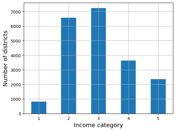
Thực hiện chia tập dữ liệu dựa trên tầng income_cat:
from sklearn.model_selection import StratifiedShuffleSplit

splitter = StratifiedShuffleSplit(n_splits=10, test_size=0.2, random_state=42)
strat_splits = []
for train_index, test_index in splitter.split(housing_full,
                                              housing_full["income_cat"]):
    strat_train_set_n = housing_full.iloc[train_index]
    strat_test_set_n = housing_full.iloc[test_index]
    strat_splits.append([strat_train_set_n, strat_test_set_n])

strat_train_set, strat_test_set = strat_splits[0]
Cách dùng train_test_split với tham số stratify gọn hơn:
strat_train_set, strat_test_set = train_test_split(
    housing_full, test_size=0.2, stratify=housing_full["income_cat"],
    random_state=42)
Kiểm tra tỷ lệ phân phối trong tập test:
strat_test_set["income_cat"].value_counts() / len(strat_test_set)output:
income_cat
3 0.350533
2 0.318798
4 0.176357
5 0.114341
1 0.039971
Name: count, dtype: float64Bảng dưới đây chứng minh rằng lấy mẫu phân tầng (Stratified) có sai số thấp hơn nhiều so với lấy mẫu ngẫu nhiên (Random) khi so sánh với phân phối gốc (Overall).
# extra code – tính toán dữ liệu cho Hình 2–10
def income_cat_proportions(data):
    return data["income_cat"].value_counts() / len(data)

train_set, test_set = train_test_split(housing_full, test_size=0.2,
                                       random_state=42)

compare_props = pd.DataFrame({
    "Overall %": income_cat_proportions(housing_full),
    "Stratified %": income_cat_proportions(strat_test_set),
    "Random %": income_cat_proportions(test_set),
}).sort_index()
compare_props.index.name = "Income Category"
compare_props["Strat. Error %"] = (compare_props["Stratified %"] /
                                   compare_props["Overall %"] - 1)
compare_props["Rand. Error %"] = (compare_props["Random %"] /
                                  compare_props["Overall %"] - 1)
(compare_props * 100).round(2)
output:
Overall % Stratified % Random % Strat. Error % \
Income Category
1 3.98 4.00 4.24 0.36
2 31.88 31.88 30.74 -0.02
3 35.06 35.05 34.52 -0.01
4 17.63 17.64 18.41 0.03
5 11.44 11.43 12.09 -0.08
Rand. Error %
Income Category
1 6.45
2 -3.59
3 -1.53
4 4.42
5 5.63 Cuối cùng, xóa biến tạm income_cat:
for set_ in (strat_train_set, strat_test_set):
    set_.drop("income_cat", axis=1, inplace=True)
4. Khám phá và Trực quan hóa Dữ liệu
housing = strat_train_set.copy()4.1. Trực quan hóa Dữ liệu Địa lý
Biểu đồ phân tán tọa độ địa lý giúp ta nhận diện các cụm dân cư.
# Biểu đồ cơ bản
housing.plot(kind="scatter", x="longitude", y="latitude", grid=True)
plt.show()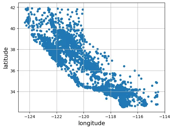
Sử dụng tham số alpha để quan sát mật độ điểm dữ liệu.
# Biểu đồ hiển thị mật độ
housing.plot(kind="scatter", x="longitude", y="latitude", grid=True, alpha=0.2)
plt.show()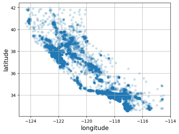
Kết hợp thông tin về dân số (kích thước s) và giá nhà (màu sắc c) giúp ta thấy rõ giá nhà cao thường tập trung ở vùng ven biển.
housing.plot(kind="scatter", x="longitude", y="latitude", grid=True,
            s=housing["population"] / 100, label="population",
            c="median_house_value", cmap="jet", colorbar=True,
            legend=True, sharex=False, figsize=(10, 7))
plt.show()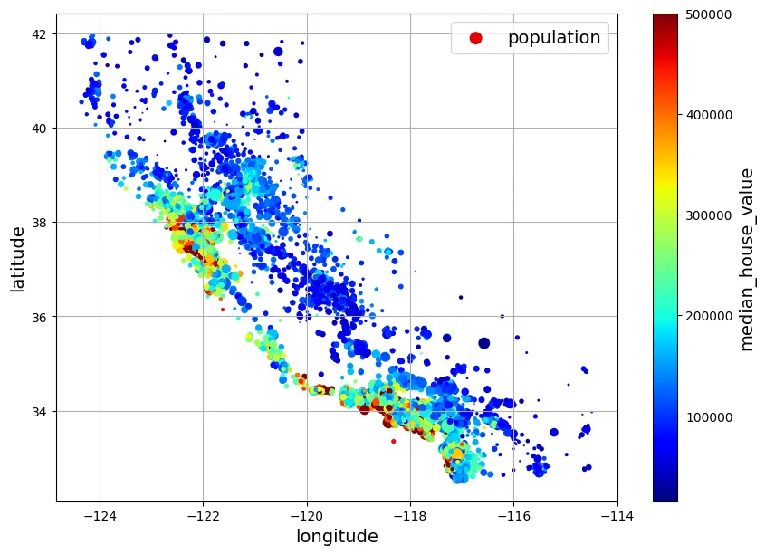
Biểu đồ nâng cao chồng lên bản đồ thực tế:
# extra code – tạo hình ảnh đầu tiên trong chương
# Tải hình ảnh bản đồ California
filename = "california.png"
filepath = Path(f"my_{filename}")
if not filepath.is_file():
    homlp_root = "https://github.com/ageron/handson-mlp/raw/main/"
    url = homlp_root + "images/end_to_end_project/" + filename
    print("Downloading", filename)
    urllib.request.urlretrieve(url, filepath)

housing_renamed = housing.rename(columns={
    "latitude": "Latitude", "longitude": "Longitude",
    "population": "Population",
    "median_house_value": "Median house value (ᴜsᴅ)"})

housing_renamed.plot(
             kind="scatter", x="Longitude", y="Latitude",
             s=housing_renamed["Population"] / 100, label="Population",
             c="Median house value (ᴜsᴅ)", cmap="jet", colorbar=True,
             legend=True, sharex=False, figsize=(10, 7))

california_img = plt.imread(filepath)
axis = -124.55, -113.95, 32.45, 42.05
plt.axis(axis)
plt.imshow(california_img, extent=axis)
plt.show()
output:
Downloading california.png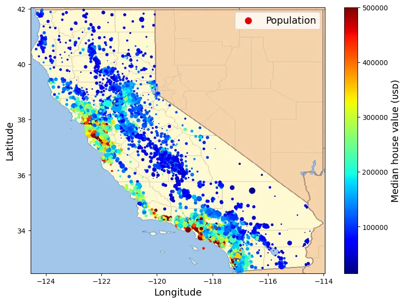
4.2. Tìm kiếm Tương quan (Correlations)
Hệ số tương quan Pearson () đo lường mối quan hệ tuyến tính giữa hai biến và :
# Tính ma trận tương quan
corr_matrix = housing.corr(numeric_only=True)corr_matrix["median_house_value"].sort_values(ascending=False)output:
median_house_value 1.000000
median_income 0.688380
total_rooms 0.137455
housing_median_age 0.102175
households 0.071426
total_bedrooms 0.054635
population -0.020153
longitude -0.050859
latitude -0.139584
Name: median_house_value, dtype: float64median_income có tương quan dương mạnh nhất () với giá nhà.
from pandas.plotting import scatter_matrix

attributes = ["median_house_value", "median_income", "total_rooms",
              "housing_median_age"]
scatter_matrix(housing[attributes], figsize=(12, 8))
plt.show()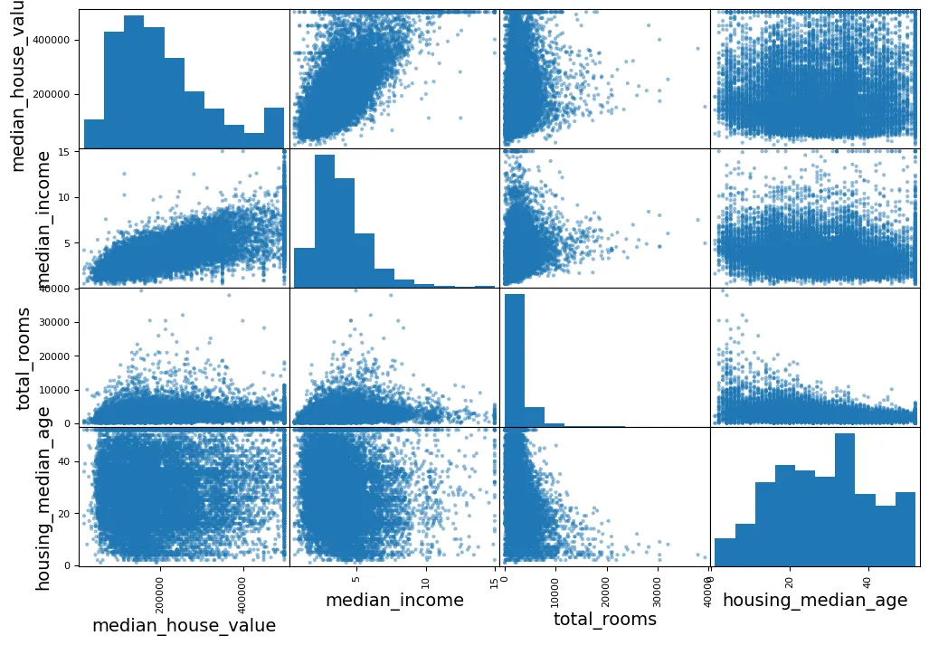
Phóng to mối quan hệ quan trọng nhất:
housing.plot(kind="scatter", x="median_income", y="median_house_value",
             alpha=0.1, grid=True)
plt.show()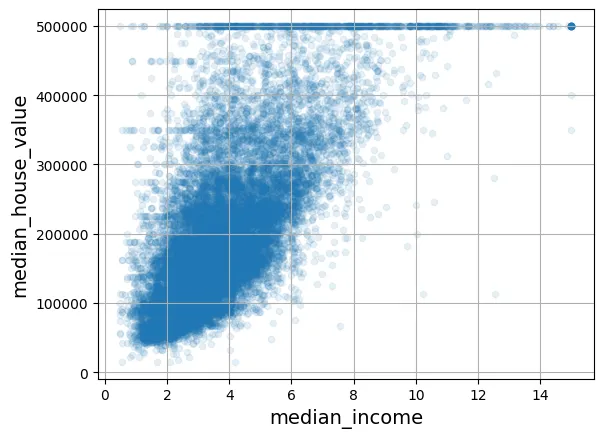
4.3. Thử nghiệm kết hợp thuộc tính (Feature Engineering)
Tạo ra các đặc trưng mới có ý nghĩa thực tiễn hơn.
housing["rooms_per_house"] = housing["total_rooms"] / housing["households"]
housing["bedrooms_ratio"] = housing["total_bedrooms"] / housing["total_rooms"]
housing["people_per_house"] = housing["population"] / housing["households"]
Kiểm tra lại tương quan, ta thấy bedrooms_ratio có tương quan âm khá tốt (), nghĩa là nhà có tỉ lệ phòng ngủ thấp thường đắt hơn.
corr_matrix = housing.corr(numeric_only=True)
corr_matrix["median_house_value"].sort_values(ascending=False)
output:
median_house_value 1.000000
median_income 0.688380
rooms_per_house 0.143663
total_rooms 0.137455
housing_median_age 0.102175
households 0.071426
total_bedrooms 0.054635
population -0.020153
people_per_house -0.038224
longitude -0.050859
latitude -0.139584
bedrooms_ratio -0.256397
Name: median_house_value, dtype: float645. Chuẩn bị Dữ liệu cho Thuật toán ML
Tách biến độc lập (X) và biến phụ thuộc (y).
housing = strat_train_set.drop("median_house_value", axis=1)
housing_labels = strat_train_set["median_house_value"].copy()
5.1. Làm sạch Dữ liệu (Data Cleaning)
Xử lý dữ liệu thiếu (Imputation).
# Mô phỏng 3 phương án (không áp dụng trực tiếp lên biến `housing` gốc ngay)
null_rows_idx = housing.isnull().any(axis=1)
housing.loc[null_rows_idx].head()

# Option 1: Xóa dòng
housing_option1 = housing.copy()
housing_option1.dropna(subset=["total_bedrooms"], inplace=True)
housing_option1.loc[null_rows_idx].head()

# Option 2: Xóa cột
housing_option2 = housing.copy()
housing_option2.drop("total_bedrooms", axis=1, inplace=True)
housing_option2.loc[null_rows_idx].head()

# Option 3: Điền giá trị trung vị (Median)
housing_option3 = housing.copy()
median = housing["total_bedrooms"].median()
housing_option3["total_bedrooms"] = housing_option3["total_bedrooms"].fillna(median)
housing_option3.loc[null_rows_idx].head()
output:
longitude latitude housing_median_age total_rooms total_bedrooms \
14452 -120.67 40.50 15.0 5343.0 434.0
18217 -117.96 34.03 35.0 2093.0 434.0
11889 -118.05 34.04 33.0 1348.0 434.0
20325 -118.88 34.17 15.0 4260.0 434.0
14360 -117.87 33.62 8.0 1266.0 434.0
population households median_income ocean_proximity
14452 2503.0 902.0 3.5962 INLAND
18217 1755.0 403.0 3.4115 <1H OCEAN
11889 1098.0 257.0 4.2917 <1H OCEAN
20325 1701.0 669.0 5.1033 <1H OCEAN
14360 375.0 183.0 9.8020 <1H OCEAN Sử dụng SimpleImputer của Scikit-Learn.
from sklearn.impute import SimpleImputer

# Khởi tạo Imputer với chiến lược là điền số trung vị
imputer = SimpleImputer(strategy="median")
housing_num = housing.select_dtypes(include=[np.number])imputer.fit(housing_num)output:
SimpleImputer(strategy='median')Các giá trị trung vị được lưu trong thuộc tính statistics_.
imputer.statistics_output:
array([-118.51 , 34.26 , 29. , 2125. , 434. , 1167. ,
408. , 3.5385])housing_num.median().valuesoutput:
array([-118.51 , 34.26 , 29. , 2125. , 434. , 1167. ,
408. , 3.5385])Biến đổi dữ liệu:
X = imputer.transform(housing_num)imputer.feature_names_in_
housing_tr = pd.DataFrame(X, columns=housing_num.columns,
index=housing_num.index)
# Kiểm tra lại các dòng từng bị thiếu
housing_tr.loc[null_rows_idx].head()output:
longitude latitude housing_median_age total_rooms total_bedrooms \
14452 -120.67 40.50 15.0 5343.0 434.0
18217 -117.96 34.03 35.0 2093.0 434.0
11889 -118.05 34.04 33.0 1348.0 434.0
20325 -118.88 34.17 15.0 4260.0 434.0
14360 -117.87 33.62 8.0 1266.0 434.0
population households median_income
14452 2503.0 902.0 3.5962
18217 1755.0 403.0 3.4115
11889 1098.0 257.0 4.2917
20325 1701.0 669.0 5.1033
14360 375.0 183.0 9.8020 imputer.strategyoutput:
'median'# Lặp lại để đảm bảo biến housing_tr có sẵn
housing_tr = pd.DataFrame(X, columns=housing_num.columns,
index=housing_num.index)
housing_tr.loc[null_rows_idx].head()output:
longitude latitude housing_median_age total_rooms total_bedrooms \
14452 -120.67 40.50 15.0 5343.0 434.0
18217 -117.96 34.03 35.0 2093.0 434.0
11889 -118.05 34.04 33.0 1348.0 434.0
20325 -118.88 34.17 15.0 4260.0 434.0
14360 -117.87 33.62 8.0 1266.0 434.0
population households median_income
14452 2503.0 902.0 3.5962
18217 1755.0 403.0 3.4115
11889 1098.0 257.0 4.2917
20325 1701.0 669.0 5.1033
14360 375.0 183.0 9.8020 # from sklearn import set_config
# set_config(transform_output="pandas") # scikit-learn >= 1.2 có thể xuất ra pandas trực tiếp5.2. Xử lý Ngoại lai (Outliers)
IsolationForest là thuật toán phát hiện bất thường dựa trên nguyên lý: các điểm dữ liệu ngoại lai dễ bị “cô lập” hơn các điểm dữ liệu bình thường.
from sklearn.ensemble import IsolationForest

isolation_forest = IsolationForest(random_state=42)
outlier_pred = isolation_forest.fit_predict(X)
outlier_pred
output:
array([-1, 1, 1, ..., 1, 1, 1])# housing = housing.iloc[outlier_pred == 1]
# housing_labels = housing_labels.iloc[outlier_pred == 1]5.3. Xử lý Đặc trưng Văn bản và Phân loại
Biến ocean_proximity là biến phân loại danh nghĩa (nominal categorical variable).
housing_cat = housing[["ocean_proximity"]]
housing_cat.head(8)
output:
ocean_proximity
13096 NEAR BAY
14973 <1H OCEAN
3785 INLAND
14689 INLAND
20507 NEAR OCEAN
1286 INLAND
18078 <1H OCEAN
4396 NEAR BAYOrdinal Encoding: Gán số thứ tự. Không phù hợp cho biến danh nghĩa không có thứ bậc (vì máy tính sẽ hiểu ).
from sklearn.preprocessing import OrdinalEncoder

ordinal_encoder = OrdinalEncoder()
housing_cat_encoded = ordinal_encoder.fit_transform(housing_cat)
housing_cat_encoded[:8]
output:
array([[3.],
[0.],
[1.],
[1.],
[4.],
[1.],
[0.],
[3.]])ordinal_encoder.categories_output:
[array(['<1H OCEAN', 'INLAND', 'ISLAND', 'NEAR BAY', 'NEAR OCEAN'],
dtype=object)]One-Hot Encoding: Tạo các vector nhị phân thưa (sparse vectors). Đây là phương pháp tiêu chuẩn cho biến danh nghĩa.
from sklearn.preprocessing import OneHotEncoder

cat_encoder = OneHotEncoder()
housing_cat_1hot = cat_encoder.fit_transform(housing_cat)
housing_cat_1hot
output:
<Compressed Sparse Row sparse matrix of dtype 'float64'
with 16512 stored elements and shape (16512, 5)>housing_cat_1hot.toarray()output:
array([[0., 0., 0., 1., 0.],
[1., 0., 0., 0., 0.],
[0., 1., 0., 0., 0.],
...,
[0., 0., 0., 0., 1.],
[1., 0., 0., 0., 0.],
[0., 0., 0., 0., 1.]])cat_encoder = OneHotEncoder(sparse_output=False)
housing_cat_1hot = cat_encoder.fit_transform(housing_cat)
housing_cat_1hotoutput:
array([[0., 0., 0., 1., 0.],
[1., 0., 0., 0., 0.],
[0., 1., 0., 0., 0.],
...,
[0., 0., 0., 0., 1.],
[1., 0., 0., 0., 0.],
[0., 0., 0., 0., 1.]])cat_encoder.categories_output:
[array(['<1H OCEAN', 'INLAND', 'ISLAND', 'NEAR BAY', 'NEAR OCEAN'],
dtype=object)]Xử lý các giá trị lạ (unknown categories) khi dự đoán:
df_test = pd.DataFrame({"ocean_proximity": ["INLAND", "NEAR BAY"]})
pd.get_dummies(df_test)
output:
ocean_proximity_INLAND ocean_proximity_NEAR BAY
0 True False
1 False Truecat_encoder.transform(df_test)output:
array([[0., 1., 0., 0., 0.],
[0., 0., 0., 1., 0.]])df_test_unknown = pd.DataFrame({"ocean_proximity": ["<2H OCEAN", "ISLAND"]})
pd.get_dummies(df_test_unknown)output:
ocean_proximity_<2H OCEAN ocean_proximity_ISLAND
0 True False
1 False Truecat_encoder.handle_unknown = "ignore"
cat_encoder.transform(df_test_unknown)output:
array([[0., 0., 0., 0., 0.],
[0., 0., 1., 0., 0.]])cat_encoder.feature_names_in_output:
array(['ocean_proximity'], dtype=object)cat_encoder.get_feature_names_out()output:
array(['ocean_proximity_<1H OCEAN', 'ocean_proximity_INLAND',
'ocean_proximity_ISLAND', 'ocean_proximity_NEAR BAY',
'ocean_proximity_NEAR OCEAN'], dtype=object)df_output = pd.DataFrame(cat_encoder.transform(df_test_unknown),
columns=cat_encoder.get_feature_names_out(),
index=df_test_unknown.index)
df_outputoutput:
ocean_proximity_<1H OCEAN ocean_proximity_INLAND ocean_proximity_ISLAND \
0 0.0 0.0 0.0
1 0.0 0.0 1.0
ocean_proximity_NEAR BAY ocean_proximity_NEAR OCEAN
0 0.0 0.0
1 0.0 0.0 5.4. Co giãn Đặc trưng (Feature Scaling)
Hầu hết các thuật toán ML (đặc biệt là dựa trên Gradient Descent) hoạt động kém khi các đặc trưng có tỷ lệ (scale) khác nhau.
- Min-Max Scaling: .
- Standardization (Chuẩn hóa): . Phương pháp này ít bị ảnh hưởng bởi ngoại lai.
from sklearn.preprocessing import MinMaxScaler

min_max_scaler = MinMaxScaler(feature_range=(-1, 1))
housing_num_min_max_scaled = min_max_scaler.fit_transform(housing_num)
from sklearn.preprocessing import StandardScaler
std_scaler = StandardScaler()
housing_num_std_scaled = std_scaler.fit_transform(housing_num)Biến đổi Logarit giúp phân phối đuôi dài trở nên gần với phân phối chuẩn hơn.
# extra code – tạo hình Figure 2–17
fig, axs = plt.subplots(1, 2, figsize=(8, 3), sharey=True)
housing["population"].hist(ax=axs[0], bins=50)
housing["population"].apply(np.log).hist(ax=axs[1], bins=50)
axs[0].set_xlabel("Population")
axs[1].set_xlabel("Log of population")
axs[0].set_ylabel("Number of districts")
plt.show()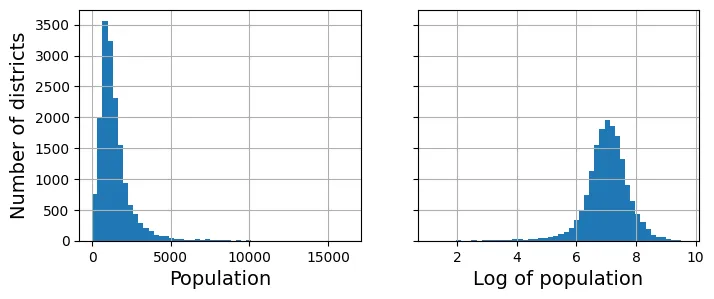
# extra code – minh họa phân phối đồng nhất (uniform) sau khi đổi sang phân vị
percentiles = [np.percentile(housing["median_income"], p)
               for p in range(1, 100)]
flattened_median_income = pd.cut(housing["median_income"],
                                 bins=[-np.inf] + percentiles + [np.inf],
                                 labels=range(1, 100 + 1))
flattened_median_income.hist(bins=50)
plt.xlabel("Median income percentile")
plt.ylabel("Number of districts")
plt.show()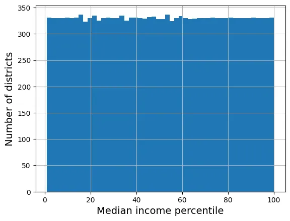
Sử dụng Radial Basis Function (RBF) Kernel để đo độ tương đồng địa lý.
from sklearn.metrics.pairwise import rbf_kernel

age_simil_35 = rbf_kernel(housing[["housing_median_age"]], [[35]], gamma=0.1)
# extra code – tạo Hình 2–18
ages = np.linspace(housing["housing_median_age"].min(),
housing["housing_median_age"].max(),
500).reshape(-1, 1)
gamma1 = 0.1
gamma2 = 0.03
rbf1 = rbf_kernel(ages, [[35]], gamma=gamma1)
rbf2 = rbf_kernel(ages, [[35]], gamma=gamma2)
fig, ax1 = plt.subplots()
ax1.set_xlabel("Housing median age")
ax1.set_ylabel("Number of districts")
ax1.hist(housing["housing_median_age"], bins=50)
ax2 = ax1.twinx() # tạo trục y thứ hai dùng chung trục x
color = "blue"
ax2.plot(ages, rbf1, color=color, label="gamma = 0.10")
ax2.plot(ages, rbf2, color=color, label="gamma = 0.03", linestyle="--")
ax2.tick_params(axis='y', labelcolor=color)
ax2.set_ylabel("Age similarity", color=color)
plt.legend(loc="upper left")
plt.show()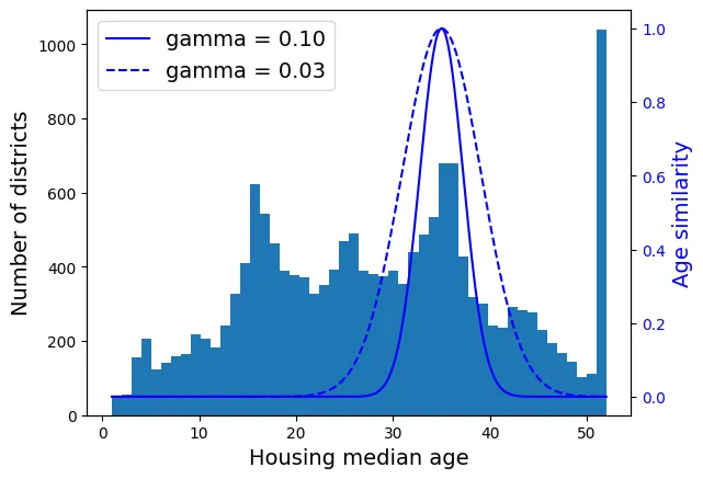
Biến đổi biến mục tiêu (target variable):
from sklearn.linear_model import LinearRegression

target_scaler = StandardScaler()
scaled_labels = target_scaler.fit_transform(housing_labels.to_frame())

model = LinearRegression()
model.fit(housing[["median_income"]], scaled_labels)
some_new_data = housing[["median_income"]].iloc[:5]
scaled_predictions = model.predict(some_new_data)
predictions = target_scaler.inverse_transform(scaled_predictions)
predictions
output:
array([[131997.15275877],
[299359.35844434],
[146023.37185694],
[138840.33653057],
[192016.61557639]])from sklearn.compose import TransformedTargetRegressor
model = TransformedTargetRegressor(LinearRegression(),
transformer=StandardScaler())
model.fit(housing[["median_income"]], housing_labels)
predictions = model.predict(some_new_data)
predictionsoutput:
array([131997.15275877, 299359.35844434, 146023.37185694, 138840.33653057,
192016.61557639])5.5. Bộ biến đổi tùy chỉnh (Custom Transformers)
from sklearn.preprocessing import FunctionTransformer

log_transformer = FunctionTransformer(np.log, inverse_func=np.exp)
log_pop = log_transformer.transform(housing[["population"]])
rbf_transformer = FunctionTransformer(rbf_kernel,
kw_args=dict(Y=[[35.]], gamma=0.1))
age_simil_35 = rbf_transformer.transform(housing[["housing_median_age"]])
age_simil_35output:
array([[2.81118530e-13],
[8.20849986e-02],
[6.70320046e-01],
...,
[9.55316054e-22],
[6.70320046e-01],
[3.03539138e-04]])sf_coords = 37.7749, -122.41
sf_transformer = FunctionTransformer(rbf_kernel,
kw_args=dict(Y=[sf_coords], gamma=0.1))
sf_simil = sf_transformer.transform(housing[["latitude", "longitude"]])
sf_similoutput:
array([[0.999927 ],
[0.05258419],
[0.94864161],
...,
[0.00388525],
[0.05038518],
[0.99868067]])ratio_transformer = FunctionTransformer(lambda X: X[:, [0]] / X[:, [1]])
ratio_transformer.transform(np.array([[1., 2.], [3., 4.]]))output:
array([[0.5 ],
[0.75]])Xây dựng Class Transformer tương thích với Scikit-Learn (kế thừa BaseEstimator, TransformerMixin).
from sklearn.base import BaseEstimator, TransformerMixin
from sklearn.utils.validation import check_array, check_is_fitted

class StandardScalerClone(BaseEstimator, TransformerMixin):
    def __init__(self, with_mean=True):  # không dùng *args hay **kwargs!
        self.with_mean = with_mean

    def fit(self, X, y=None):  # y là bắt buộc dù không dùng
        X = check_array(X)  # kiểm tra X là mảng hợp lệ
        self.mean_ = X.mean(axis=0)
        self.scale_ = X.std(axis=0)
        self.n_features_in_ = X.shape[1]
        return self  # luôn trả về self!

    def transform(self, X):
        check_is_fitted(self)  # kiểm tra xem đã fit chưa
        X = check_array(X)
        assert self.n_features_in_ == X.shape[1]
        if self.with_mean:
            X = X - self.mean_
        return X / self.scale_
Transformer sử dụng K-Means để tạo đặc trưng cụm (clustering features).
from sklearn.cluster import KMeans

class ClusterSimilarity(BaseEstimator, TransformerMixin):
    def __init__(self, n_clusters=10, gamma=1.0, random_state=None):
        self.n_clusters = n_clusters
        self.gamma = gamma
        self.random_state = random_state

    def fit(self, X, y=None, sample_weight=None):
        self.kmeans_ = KMeans(self.n_clusters, random_state=self.random_state)
        self.kmeans_.fit(X, sample_weight=sample_weight)
        return self

    def transform(self, X):
        return rbf_kernel(X, self.kmeans_.cluster_centers_, gamma=self.gamma)

    def get_feature_names_out(self, names=None):
        return [f"Cluster {i} similarity" for i in range(self.n_clusters)]
cluster_simil = ClusterSimilarity(n_clusters=10, gamma=1., random_state=42)
similarities = cluster_simil.fit_transform(housing[["latitude", "longitude"]])
similarities[:3].round(2)output:
array([[0.46, 0. , 0.08, 0. , 0. , 0. , 0. , 0.98, 0. , 0. ],
[0. , 0.96, 0. , 0.03, 0.04, 0. , 0. , 0. , 0.11, 0.35],
[0.34, 0. , 0.45, 0. , 0. , 0. , 0.01, 0.73, 0. , 0. ]])# extra code – tạo Hình 2–19
housing_renamed = housing.rename(columns={
"latitude": "Latitude", "longitude": "Longitude",
"population": "Population",
"median_house_value": "Median house value (ᴜsᴅ)"})
housing_renamed["Max cluster similarity"] = similarities.max(axis=1)
housing_renamed.plot(kind="scatter", x="Longitude", y="Latitude", grid=True,
s=housing_renamed["Population"] / 100, label="Population",
c="Max cluster similarity",
cmap="jet", colorbar=True,
legend=True, sharex=False, figsize=(10, 7))
plt.plot(cluster_simil.kmeans_.cluster_centers_[:, 1],
cluster_simil.kmeans_.cluster_centers_[:, 0],
linestyle="", color="black", marker="X", markersize=20,
label="Cluster centers")
plt.legend(loc="upper right")
plt.show()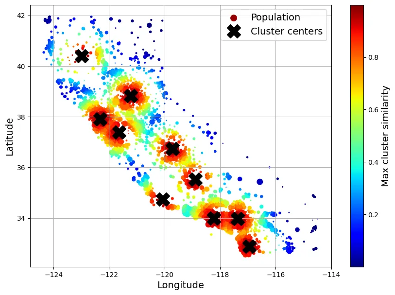
5.6. Pipeline Chuyển đổi (Transformation Pipelines)
Pipeline giúp xâu chuỗi các bước xử lý, tránh rò rỉ dữ liệu (data leakage).
from sklearn.pipeline import Pipeline

num_pipeline = Pipeline([
    ("impute", SimpleImputer(strategy="median")),
    ("standardize", StandardScaler()),
])
from sklearn.pipeline import make_pipeline
num_pipeline = make_pipeline(SimpleImputer(strategy="median"), StandardScaler())from sklearn import set_config
set_config(display='diagram')
num_pipelineoutput:
Pipeline(steps=[('simpleimputer', SimpleImputer(strategy='median')),
('standardscaler', StandardScaler())])housing_num_prepared = num_pipeline.fit_transform(housing_num)
housing_num_prepared[:2].round(2)output:
array([[-1.42, 1.01, 1.86, 0.31, 1.37, 0.14, 1.39, -0.94],
[ 0.6 , -0.7 , 0.91, -0.31, -0.44, -0.69, -0.37, 1.17]])df_housing_num_prepared = pd.DataFrame(
housing_num_prepared, columns=num_pipeline.get_feature_names_out(),
index=housing_num.index)
df_housing_num_prepared.head(2)output:
longitude latitude housing_median_age total_rooms total_bedrooms \
13096 -1.423037 1.013606 1.861119 0.311912 1.368167
14973 0.596394 -0.702103 0.907630 -0.308620 -0.435925
population households median_income
13096 0.137460 1.394812 -0.936491
14973 -0.693771 -0.373485 1.171942 num_pipeline.steps
num_pipeline[1]
num_pipeline[:-1]
num_pipeline.named_steps["simpleimputer"]
num_pipeline.set_params(simpleimputer__strategy="median")output:
Pipeline(steps=[('simpleimputer', SimpleImputer(strategy='median')),
('standardscaler', StandardScaler())])ColumnTransformer xử lý song song các cột dữ liệu khác nhau (số và phân loại).
from sklearn.compose import ColumnTransformer

num_attribs = ["longitude", "latitude", "housing_median_age", "total_rooms",
               "total_bedrooms", "population", "households", "median_income"]
cat_attribs = ["ocean_proximity"]

cat_pipeline = make_pipeline(
    SimpleImputer(strategy="most_frequent"),
    OneHotEncoder(handle_unknown="ignore"))

preprocessing = ColumnTransformer([
    ("num", num_pipeline, num_attribs),
    ("cat", cat_pipeline, cat_attribs),
])
from sklearn.compose import make_column_selector, make_column_transformer
preprocessing = make_column_transformer(
(num_pipeline, make_column_selector(dtype_include=np.number)),
(cat_pipeline, make_column_selector(dtype_include=object)),
)housing_prepared = preprocessing.fit_transform(housing)
# extra code – chuyển về DataFrame
housing_prepared_fr = pd.DataFrame(
housing_prepared,
columns=preprocessing.get_feature_names_out(),
index=housing.index)
housing_prepared_fr.head(2)output:
pipeline-1__longitude pipeline-1__latitude \
13096 -1.423037 1.013606
14973 0.596394 -0.702103
pipeline-1__housing_median_age pipeline-1__total_rooms \
13096 1.861119 0.311912
14973 0.907630 -0.308620
pipeline-1__total_bedrooms pipeline-1__population \
13096 1.368167 0.137460
14973 -0.435925 -0.693771
pipeline-1__households pipeline-1__median_income \
13096 1.394812 -0.936491
14973 -0.373485 1.171942
pipeline-2__ocean_proximity_<1H OCEAN \
13096 0.0
14973 1.0
pipeline-2__ocean_proximity_INLAND pipeline-2__ocean_proximity_ISLAND \
13096 0.0 0.0
14973 0.0 0.0
pipeline-2__ocean_proximity_NEAR BAY \
13096 1.0
14973 0.0
pipeline-2__ocean_proximity_NEAR OCEAN
13096 0.0
14973 0.0 Pipeline hoàn chỉnh (Full Pipeline):
def column_ratio(X):
    return X[:, [0]] / X[:, [1]]

def ratio_name(function_transformer, feature_names_in):
    return ["ratio"]

def ratio_pipeline():
    return make_pipeline(
        SimpleImputer(strategy="median"),
        FunctionTransformer(column_ratio, feature_names_out=ratio_name),
        StandardScaler())

log_pipeline = make_pipeline(
    SimpleImputer(strategy="median"),
    FunctionTransformer(np.log, feature_names_out="one-to-one"),
    StandardScaler())

cluster_simil = ClusterSimilarity(n_clusters=10, gamma=1., random_state=42)
default_num_pipeline = make_pipeline(SimpleImputer(strategy="median"),
                                     StandardScaler())

preprocessing = ColumnTransformer([
        ("bedrooms", ratio_pipeline(), ["total_bedrooms", "total_rooms"]),
        ("rooms_per_house", ratio_pipeline(), ["total_rooms", "households"]),
        ("people_per_house", ratio_pipeline(), ["population", "households"]),
        ("log", log_pipeline, ["total_bedrooms", "total_rooms", "population",
                               "households", "median_income"]),
        ("geo", cluster_simil, ["latitude", "longitude"]),
        ("cat", cat_pipeline, make_column_selector(dtype_include=object)),
    ],
    remainder=default_num_pipeline)  # cột còn lại: housing_median_age

housing_prepared = preprocessing.fit_transform(housing)
housing_prepared.shape
output:
(16512, 24)preprocessing.get_feature_names_out()output:
array(['bedrooms__ratio', 'rooms_per_house__ratio',
'people_per_house__ratio', 'log__total_bedrooms',
'log__total_rooms', 'log__population', 'log__households',
'log__median_income', 'geo__Cluster 0 similarity',
'geo__Cluster 1 similarity', 'geo__Cluster 2 similarity',
'geo__Cluster 3 similarity', 'geo__Cluster 4 similarity',
'geo__Cluster 5 similarity', 'geo__Cluster 6 similarity',
'geo__Cluster 7 similarity', 'geo__Cluster 8 similarity',
'geo__Cluster 9 similarity', 'cat__ocean_proximity_<1H OCEAN',
'cat__ocean_proximity_INLAND', 'cat__ocean_proximity_ISLAND',
'cat__ocean_proximity_NEAR BAY', 'cat__ocean_proximity_NEAR OCEAN',
'remainder__housing_median_age'], dtype=object)6. Lựa chọn và Huấn luyện Mô hình
6.1. Huấn luyện và Đánh giá trên Tập Huấn luyện
Mô hình đầu tiên: Hồi quy Tuyến tính (Linear Regression). Hàm mất mát (Cost function) là Mean Squared Error (MSE):
from sklearn.linear_model import LinearRegression

lin_reg = make_pipeline(preprocessing, LinearRegression())
lin_reg.fit(housing, housing_labels)
output:
Pipeline(steps=[('columntransformer',
ColumnTransformer(remainder=Pipeline(steps=[('simpleimputer',
SimpleImputer(strategy='median')),
('standardscaler',
StandardScaler())]),
transformers=[('bedrooms',
Pipeline(steps=[('simpleimputer',
SimpleImputer(strategy='median')),
('functiontransformer',
FunctionTransformer(feature_names_out=<function ratio_name at 0x7e2...
'median_income']),
('geo',
ClusterSimilarity(random_state=42),
['latitude', 'longitude']),
('cat',
Pipeline(steps=[('simpleimputer',
SimpleImputer(strategy='most_frequent')),
('onehotencoder',
OneHotEncoder(handle_unknown='ignore'))]),
<sklearn.compose._column_transformer.make_column_selector object at 0x7e2b87d49940>)])),
('linearregression', LinearRegression())])housing_predictions = lin_reg.predict(housing)
housing_predictions[:5].round(-2)output:
array([246000., 372700., 135700., 91400., 330900.])housing_labels.iloc[:5].valuesoutput:
array([458300., 483800., 101700., 96100., 361800.])# extra code – tính tỷ lệ lỗi
error_ratios = housing_predictions[:5].round(-2) / housing_labels.iloc[:5].values - 1
print(", ".join([f"{100 * ratio:.1f}%" for ratio in error_ratios]))output:
-46.3%, -23.0%, 33.4%, -4.9%, -8.5%Sử dụng RMSE (Root Mean Squared Error) làm thước đo hiệu suất:
from sklearn.metrics import root_mean_squared_error

lin_rmse = root_mean_squared_error(housing_labels, housing_predictions)
lin_rmse
output:
68972.88910758484RMSE xấp xỉ 69,000 USD. So với khoảng giá nhà (120k - 265k USD), sai số này là lớn -> Underfitting.
Thử mô hình phức tạp hơn: Decision Tree Regressor.
from sklearn.tree import DecisionTreeRegressor

tree_reg = make_pipeline(preprocessing, DecisionTreeRegressor(random_state=42))
tree_reg.fit(housing, housing_labels)
output:
Pipeline(steps=[('columntransformer',
ColumnTransformer(remainder=Pipeline(steps=[('simpleimputer',
SimpleImputer(strategy='median')),
('standardscaler',
StandardScaler())]),
transformers=[('bedrooms',
Pipeline(steps=[('simpleimputer',
SimpleImputer(strategy='median')),
('functiontransformer',
FunctionTransformer(feature_names_out=<function ratio_name at 0x7e2...
ClusterSimilarity(random_state=42),
['latitude', 'longitude']),
('cat',
Pipeline(steps=[('simpleimputer',
SimpleImputer(strategy='most_frequent')),
('onehotencoder',
OneHotEncoder(handle_unknown='ignore'))]),
<sklearn.compose._column_transformer.make_column_selector object at 0x7e2b87d49940>)])),
('decisiontreeregressor',
DecisionTreeRegressor(random_state=42))])housing_predictions = tree_reg.predict(housing)
tree_rmse = root_mean_squared_error(housing_labels, housing_predictions)
tree_rmseoutput:
0.0RMSE = 0.0? Mô hình hoàn hảo? Không, đây là dấu hiệu của Overfitting (Quá khớp) trên tập huấn luyện.
6.2. Đánh giá tốt hơn bằng Cross-Validation
K-Fold Cross-Validation giúp ước lượng lỗi tổng quát hóa (generalization error).
from sklearn.model_selection import cross_val_score

tree_rmses = -cross_val_score(tree_reg, housing, housing_labels,
                              scoring="neg_root_mean_squared_error", cv=10)
pd.Series(tree_rmses).describe()
output:
count 10.000000
mean 66573.734600
std 1103.402323
min 64607.896046
25% 66204.731788
50% 66388.272499
75% 66826.257468
max 68532.210664
dtype: float64RMSE trung bình của Decision Tree là ~66,573, thực sự tệ hơn cả Linear Regression.
# extra code
lin_rmses = -cross_val_score(lin_reg, housing, housing_labels,
                              scoring="neg_root_mean_squared_error", cv=10)
pd.Series(lin_rmses).describe()
output:
count 10.000000
mean 70003.404818
std 4182.188328
min 65504.765753
25% 68172.065831
50% 68743.995249
75% 70344.943988
max 81037.863741
dtype: float64Thử nghiệm Random Forest Regressor - thuật toán Ensemble Learning.
from sklearn.ensemble import RandomForestRegressor

forest_reg = make_pipeline(preprocessing,
                           RandomForestRegressor(random_state=42))
forest_rmses = -cross_val_score(forest_reg, housing, housing_labels,
                                scoring="neg_root_mean_squared_error", cv=10)
pd.Series(forest_rmses).describe()
output:
count 10.000000
mean 47038.092799
std 1021.491757
min 45495.976649
25% 46510.418013
50% 47118.719249
75% 47480.519175
max 49140.832210
dtype: float64forest_reg.fit(housing, housing_labels)
housing_predictions = forest_reg.predict(housing)
forest_rmse = root_mean_squared_error(housing_labels, housing_predictions)
forest_rmseoutput:
17551.2122500877Random Forest cho kết quả tốt hơn nhiều (47k vs 66k). Tuy nhiên, lỗi trên tập train (17.5k) thấp hơn nhiều so với validation (47k) -> vẫn còn Overfitting.
7. Tinh chỉnh Mô hình (Fine-Tuning)
7.1. Tìm kiếm Lưới (Grid Search)
Duyệt qua không gian siêu tham số (Hyperparameter space) một cách có hệ thống.
from sklearn.model_selection import GridSearchCV

full_pipeline = Pipeline([
    ("preprocessing", preprocessing),
    ("random_forest", RandomForestRegressor(random_state=42)),
])

param_grid = [
    {'preprocessing__geo__n_clusters': [5, 8, 10],
     'random_forest__max_features': [4, 6, 8]},
    {'preprocessing__geo__n_clusters': [10, 15],
     'random_forest__max_features': [6, 8, 10]},
]

grid_search = GridSearchCV(full_pipeline, param_grid, cv=3,
                           scoring='neg_root_mean_squared_error')
grid_search.fit(housing, housing_labels)
output:
GridSearchCV(cv=3,
estimator=Pipeline(steps=[('preprocessing',
ColumnTransformer(remainder=Pipeline(steps=[('simpleimputer',
SimpleImputer(strategy='median')),
('standardscaler',
StandardScaler())]),
transformers=[('bedrooms',
Pipeline(steps=[('simpleimputer',
SimpleImputer(strategy='median')),
('functiontransformer',
FunctionTransformer(feature_names_out=<f...
<sklearn.compose._column_transformer.make_column_selector object at 0x7e2b87d49940>)])),
('random_forest',
RandomForestRegressor(random_state=42))]),
param_grid=[{'preprocessing__geo__n_clusters': [5, 8, 10],
'random_forest__max_features': [4, 6, 8]},
{'preprocessing__geo__n_clusters': [10, 15],
'random_forest__max_features': [6, 8, 10]}],
scoring='neg_root_mean_squared_error')# extra code – hiển thị một phần output của get_params().keys()
print(str(full_pipeline.get_params().keys())[:1000] + "...")output:
dict_keys(['memory', 'steps', 'transform_input', 'verbose', 'preprocessing', 'random_forest', 'preprocessing__force_int_remainder_cols', 'preprocessing__n_jobs', 'preprocessing__remainder__memory', 'preprocessing__remainder__steps', 'preprocessing__remainder__transform_input', 'preprocessing__remainder__verbose', 'preprocessing__remainder__simpleimputer', 'preprocessing__remainder__standardscaler', 'preprocessing__remainder__simpleimputer__add_indicator', 'preprocessing__remainder__simpleimputer__copy', 'preprocessing__remainder__simpleimputer__fill_value', 'preprocessing__remainder__simpleimputer__keep_empty_features', 'preprocessing__remainder__simpleimputer__missing_values', 'preprocessing__remainder__simpleimputer__strategy', 'preprocessing__remainder__standardscaler__copy', 'preprocessing__remainder__standardscaler__with_mean', 'preprocessing__remainder__standardscaler__with_std', 'preprocessing__remainder', 'preprocessing__sparse_threshold', 'preprocessing__transformer_weights', ...grid_search.best_params_output:
{'preprocessing__geo__n_clusters': 15, 'random_forest__max_features': 6}grid_search.best_estimator_output:
Pipeline(steps=[('preprocessing',
ColumnTransformer(remainder=Pipeline(steps=[('simpleimputer',
SimpleImputer(strategy='median')),
('standardscaler',
StandardScaler())]),
transformers=[('bedrooms',
Pipeline(steps=[('simpleimputer',
SimpleImputer(strategy='median')),
('functiontransformer',
FunctionTransformer(feature_names_out=<function ratio_name at 0x7e2b87d...
ClusterSimilarity(n_clusters=15,
random_state=42),
['latitude', 'longitude']),
('cat',
Pipeline(steps=[('simpleimputer',
SimpleImputer(strategy='most_frequent')),
('onehotencoder',
OneHotEncoder(handle_unknown='ignore'))]),
<sklearn.compose._column_transformer.make_column_selector object at 0x7e2b8a422270>)])),
('random_forest',
RandomForestRegressor(max_features=6, random_state=42))])cv_res = pd.DataFrame(grid_search.cv_results_)
cv_res.sort_values(by="mean_test_score", ascending=False, inplace=True)
# extra code – làm đẹp bảng kết quả
cv_res = cv_res[["param_preprocessing__geo__n_clusters",
"param_random_forest__max_features", "split0_test_score",
"split1_test_score", "split2_test_score", "mean_test_score"]]
score_cols = ["split0", "split1", "split2", "mean_test_rmse"]
cv_res.columns = ["n_clusters", "max_features"] + score_cols
cv_res[score_cols] = -cv_res[score_cols].round().astype(np.int64)
cv_res.head()output:
n_clusters max_features split0 split1 split2 mean_test_rmse
12 15 6 42725 43708 44335 43590
13 15 8 43486 43820 44900 44069
6 10 4 43798 44036 44961 44265
9 10 6 43710 44163 44967 44280
7 10 6 43710 44163 44967 442807.2. Tìm kiếm Ngẫu nhiên (Randomized Search)
Khi không gian tham số lớn, Randomized Search hiệu quả hơn.
from sklearn.experimental import enable_halving_search_cv
from sklearn.model_selection import HalvingRandomSearchCV
from sklearn.model_selection import RandomizedSearchCV
from scipy.stats import randint
param_distribs = {'preprocessing__geo__n_clusters': randint(low=3, high=50),
'random_forest__max_features': randint(low=2, high=20)}
rnd_search = RandomizedSearchCV(
full_pipeline, param_distributions=param_distribs, n_iter=10, cv=3,
scoring='neg_root_mean_squared_error', random_state=42)
rnd_search.fit(housing, housing_labels)output:
RandomizedSearchCV(cv=3,
estimator=Pipeline(steps=[('preprocessing',
ColumnTransformer(remainder=Pipeline(steps=[('simpleimputer',
SimpleImputer(strategy='median')),
('standardscaler',
StandardScaler())]),
transformers=[('bedrooms',
Pipeline(steps=[('simpleimputer',
SimpleImputer(strategy='median')),
('functiontransformer',
FunctionTransformer(feature_names_...
('random_forest',
RandomForestRegressor(random_state=42))]),
param_distributions={'preprocessing__geo__n_clusters': <scipy.stats._distn_infrastructure.rv_discrete_frozen object at 0x7e2b87d4ac60>,
'random_forest__max_features': <scipy.stats._distn_infrastructure.rv_discrete_frozen object at 0x7e2b8b770ce0>},
random_state=42, scoring='neg_root_mean_squared_error')# extra code – hiển thị kết quả random search
cv_res = pd.DataFrame(rnd_search.cv_results_)
cv_res.sort_values(by="mean_test_score", ascending=False, inplace=True)
cv_res = cv_res[["param_preprocessing__geo__n_clusters",
"param_random_forest__max_features", "split0_test_score",
"split1_test_score", "split2_test_score", "mean_test_score"]]
cv_res.columns = ["n_clusters", "max_features"] + score_cols
cv_res[score_cols] = -cv_res[score_cols].round().astype(np.int64)
cv_res.head()output:
n_clusters max_features split0 split1 split2 mean_test_rmse
1 45 9 41342 42242 43057 42214
8 32 7 41825 42275 43241 42447
0 41 16 42238 42938 43354 42843
5 42 4 41869 43362 43664 42965
2 23 8 42490 42928 43718 43046Lựa chọn phân phối xác suất cho tham số: randint (đồng nhất rời rạc) vs loguniform (logarit đồng nhất - thích hợp khi ta không biết quy mô của tham số).
# extra code – vẽ biểu đồ minh họa các phân phối xác suất
from scipy.stats import randint, uniform, geom, expon

xs1 = np.arange(0, 7 + 1)
randint_distrib = randint(0, 7 + 1).pmf(xs1)

xs2 = np.linspace(0, 7, 500)
uniform_distrib = uniform(0, 7).pdf(xs2)

xs3 = np.arange(0, 7 + 1)
geom_distrib = geom(0.5).pmf(xs3)

xs4 = np.linspace(0, 7, 500)
expon_distrib = expon(scale=1).pdf(xs4)

plt.figure(figsize=(12, 7))
plt.subplot(2, 2, 1)
plt.bar(xs1, randint_distrib, label="scipy.randint(0, 7 + 1)")
plt.ylabel("Probability")
plt.legend()
plt.axis([-1, 8, 0, 0.2])

plt.subplot(2, 2, 2)
plt.fill_between(xs2, uniform_distrib, label="scipy.uniform(0, 7)")
plt.ylabel("PDF")
plt.legend()
plt.axis([-1, 8, 0, 0.2])

plt.subplot(2, 2, 3)
plt.bar(xs3, geom_distrib, label="scipy.geom(0.5)")
plt.xlabel("Hyperparameter value")
plt.ylabel("Probability")
plt.legend()
plt.axis([0, 7, 0, 1])

plt.subplot(2, 2, 4)
plt.fill_between(xs4, expon_distrib, label="scipy.expon(scale=1)")
plt.xlabel("Hyperparameter value")
plt.ylabel("PDF")
plt.legend()
plt.axis([0, 7, 0, 1])

plt.show()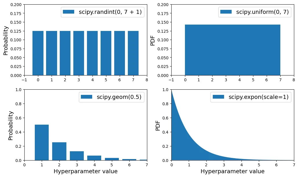
# extra code – so sánh expon và loguniform
from scipy.stats import loguniform

xs1 = np.linspace(0, 7, 500)
expon_distrib = expon(scale=1).pdf(xs1)

log_xs2 = np.linspace(-5, 3, 500)
log_expon_distrib = np.exp(log_xs2 - np.exp(log_xs2))

xs3 = np.linspace(0.001, 1000, 500)
loguniform_distrib = loguniform(0.001, 1000).pdf(xs3)

log_xs4 = np.linspace(np.log(0.001), np.log(1000), 500)
log_loguniform_distrib = uniform(np.log(0.001), np.log(1000)).pdf(log_xs4)

plt.figure(figsize=(12, 7))
plt.subplot(2, 2, 1)
plt.fill_between(xs1, expon_distrib,
                 label="scipy.expon(scale=1)")
plt.ylabel("PDF")
plt.legend()
plt.axis([0, 7, 0, 1])

plt.subplot(2, 2, 2)
plt.fill_between(log_xs2, log_expon_distrib,
                 label="log(X) with X ~ expon")
plt.legend()
plt.axis([-5, 3, 0, 1])

plt.subplot(2, 2, 3)
plt.fill_between(xs3, loguniform_distrib,
                 label="scipy.loguniform(0.001, 1000)")
plt.xlabel("Hyperparameter value")
plt.ylabel("PDF")
plt.legend()
plt.axis([0.001, 1000, 0, 0.005])

plt.subplot(2, 2, 4)
plt.fill_between(log_xs4, log_loguniform_distrib,
                 label="log(X) with X ~ loguniform")
plt.xlabel("Log of hyperparameter value")
plt.legend()
plt.axis([-8, 1, 0, 0.2])
plt.show()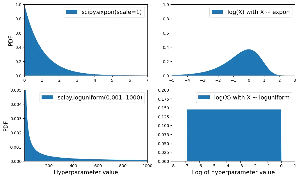
7.3. Phân tích Mô hình Tốt nhất (Analyze Best Model)
Đánh giá độ quan trọng của đặc trưng (Feature Importance).
final_model = rnd_search.best_estimator_  # bao gồm cả preprocessing
feature_importances = final_model["random_forest"].feature_importances_
feature_importances.round(2)
output:
array([0.07, 0.05, 0.05, 0.01, 0.01, 0.01, 0.01, 0.19, 0.01, 0.02, 0.01,
0.01, 0.01, 0. , 0.01, 0.02, 0.01, 0.02, 0.01, 0. , 0.01, 0.02,
0.01, 0.01, 0.01, 0. , 0.02, 0.01, 0.01, 0. , 0.01, 0.01, 0.01,
0.03, 0.01, 0.01, 0.01, 0.01, 0.04, 0.01, 0.02, 0.01, 0.02, 0.01,
0.02, 0.02, 0.01, 0.01, 0.01, 0.01, 0.01, 0.01, 0.01, 0. , 0.07,
0. , 0. , 0. , 0.01])sorted(zip(feature_importances,
final_model["preprocessing"].get_feature_names_out()),
reverse=True)output:
[(np.float64(0.18599734460509476), 'log__median_income'),
(np.float64(0.07338850855844489), 'cat__ocean_proximity_INLAND'),
(np.float64(0.06556941990883976), 'bedrooms__ratio'),
(np.float64(0.053648710076725316), 'rooms_per_house__ratio'),
(np.float64(0.04598870861894749), 'people_per_house__ratio'),
...
]log__median_income là yếu tố quan trọng nhất.
7.4. Đánh giá trên Tập Kiểm tra (Final Evaluation)
X_test = strat_test_set.drop("median_house_value", axis=1)
y_test = strat_test_set["median_house_value"].copy()

final_predictions = final_model.predict(X_test)

final_rmse = root_mean_squared_error(y_test, final_predictions)
print(final_rmse)
output:
41445.533268606625Tính Khoảng tin cậy (Confidence Interval) 95% cho RMSE bằng phương pháp Bootstrap.
from scipy.stats import bootstrap

def rmse(squared_errors):
    return np.sqrt(np.mean(squared_errors))

confidence = 0.95
squared_errors = (final_predictions - y_test) ** 2
boot_result = bootstrap([squared_errors], rmse, confidence_level=confidence,
                        random_state=42)
rmse_lower, rmse_upper = boot_result.confidence_interval
print(f"95% CI for RMSE: ({rmse_lower:.4f}, {rmse_upper:.4f})")
output:
95% CI for RMSE: (39520.9572, 43701.7681)8. Lưu và Triển khai Mô hình
import joblib

joblib.dump(final_model, "my_california_housing_model.pkl")
output:
['my_california_housing_model.pkl']import joblib
# extra code – định nghĩa lại các thành phần phụ thuộc nếu tải ở script khác
from sklearn.cluster import KMeans
from sklearn.base import BaseEstimator, TransformerMixin
from sklearn.metrics.pairwise import rbf_kernel
def column_ratio(X):
return X[:, [0]] / X[:, [1]]
# class ClusterSimilarity(BaseEstimator, TransformerMixin):
# [...]
final_model_reloaded = joblib.load("my_california_housing_model.pkl")
new_data = housing.iloc[:5] # giả sử đây là dữ liệu mới
predictions = final_model_reloaded.predict(new_data)
predictionsoutput:
array([441046.12, 454713.09, 104832. , 101316. , 336181.05])9. Bài tập Thực hành
Bài tập 1: Support Vector Machine (SVR)
Sử dụng Support Vector Regressor (SVR).
from sklearn.model_selection import GridSearchCV
from sklearn.svm import SVR

param_grid = [
        {'svr__kernel': ['linear'], 'svr__C': [10., 30., 100., 300., 1000.,
                                               3000., 10000., 30000.0]},
        {'svr__kernel': ['rbf'], 'svr__C': [1.0, 3.0, 10., 30., 100., 300.,
                                            1000.0],
         'svr__gamma': [0.01, 0.03, 0.1, 0.3, 1.0, 3.0]},
    ]

svr_pipeline = Pipeline([("preprocessing", preprocessing), ("svr", SVR())])

grid_search = GridSearchCV(svr_pipeline, param_grid, cv=3,
                           scoring='neg_root_mean_squared_error')
grid_search.fit(housing.iloc[:5000], housing_labels.iloc[:5000])
output:
GridSearchCV(cv=3,
estimator=Pipeline(steps=[('preprocessing',
ColumnTransformer(remainder=Pipeline(steps=[('simpleimputer',
SimpleImputer(strategy='median')),
('standardscaler',
StandardScaler())]),
transformers=[('bedrooms',
Pipeline(steps=[('simpleimputer',
SimpleImputer(strategy='median')),
('functiontransformer',
FunctionTransformer(feature_names_out=<f...
<sklearn.compose._column_transformer.make_column_selector object at 0x7e2b87d49940>)])),
('svr', SVR())]),
param_grid=[{'svr__C': [10.0, 30.0, 100.0, 300.0, 1000.0, 3000.0,
10000.0, 30000.0],
'svr__kernel': ['linear']},
{'svr__C': [1.0, 3.0, 10.0, 30.0, 100.0, 300.0,
1000.0],
'svr__gamma': [0.01, 0.03, 0.1, 0.3, 1.0, 3.0],
'svr__kernel': ['rbf']}],
scoring='neg_root_mean_squared_error')svr_grid_search_rmse = -grid_search.best_score_
svr_grid_search_rmseoutput:
np.float64(70059.9277356289)grid_search.best_params_output:
{'svr__C': 10000.0, 'svr__kernel': 'linear'}Bài tập 2: RandomizedSearchCV cho SVM
from sklearn.model_selection import RandomizedSearchCV
from scipy.stats import expon, loguniform

# Note: gamma bị bỏ qua khi kernel là "linear"
param_distribs = {
        'svr__kernel': ['linear', 'rbf'],
        'svr__C': loguniform(20, 200_000),
        'svr__gamma': expon(scale=1.0),
    }

rnd_search = RandomizedSearchCV(svr_pipeline,
                                param_distributions=param_distribs,
                                n_iter=50, cv=3,
                                scoring='neg_root_mean_squared_error',
                                random_state=42)
rnd_search.fit(housing.iloc[:5000], housing_labels.iloc[:5000])
output:
RandomizedSearchCV(cv=3,
estimator=Pipeline(steps=[('preprocessing',
ColumnTransformer(remainder=Pipeline(steps=[('simpleimputer',
SimpleImputer(strategy='median')),
('standardscaler',
StandardScaler())]),
...svr_rnd_search_rmse = -rnd_search.best_score_
svr_rnd_search_rmseoutput:
np.float64(56152.053691161)rnd_search.best_params_output:
{'svr__C': np.float64(157055.10989448498),
'svr__gamma': np.float64(0.26497040005002437),
'svr__kernel': 'rbf'}# Kiểm tra phân phối của gamma
s = expon(scale=1).rvs(100_000, random_state=42)
((s > 0.105) & (s < 2.29)).sum() / 100_000output:
np.float64(0.80066)Bài tập 3: Chọn lọc đặc trưng (SelectFromModel)
from sklearn.feature_selection import SelectFromModel

selector_pipeline = Pipeline([
    ('preprocessing', preprocessing),
    ('selector', SelectFromModel(RandomForestRegressor(random_state=42),
                                 threshold=0.005)),  # ngưỡng độ quan trọng tối thiểu
    ('svr', SVR(C=rnd_search.best_params_["svr__C"],
                gamma=rnd_search.best_params_["svr__gamma"],
                kernel=rnd_search.best_params_["svr__kernel"])),
])
selector_rmses = -cross_val_score(selector_pipeline,
housing.iloc[:5000],
housing_labels.iloc[:5000],
scoring="neg_root_mean_squared_error",
cv=3)
pd.Series(selector_rmses).describe()output:
count 3.000000
mean 56622.643481
std 2272.666703
min 54243.242290
25% 55548.509493
50% 56853.776696
75% 57812.344076
max 58770.911457
dtype: float64Bài tập 4: Transformer tùy chỉnh dùng KNN
from sklearn.base import MetaEstimatorMixin, clone

class FeatureFromRegressor(BaseEstimator, TransformerMixin, MetaEstimatorMixin):
    def __init__(self, regressor, target_features):
        self.regressor = regressor
        self.target_features = target_features

    def fit(self, X, y=None):
        if hasattr(X, "columns"):
            self.feature_names_in_ = list(X.columns)
            X_df = X
        else:
            X_df = pd.DataFrame(X)

        self.input_features_ = [c for c in X_df.columns
                                if c not in self.target_features]
        self.regressor_ = clone(self.regressor)
        self.regressor_.fit(X_df[self.input_features_],
                            X_df[self.target_features])
        return self

    def transform(self, X):
        columns = X.columns if hasattr(X, "columns") else None
        X_df = pd.DataFrame(X, columns=columns)
        preds = self.regressor_.predict(X_df[self.input_features_])
        if preds.ndim == 1:
            preds = preds.reshape(-1, 1)
        extra_columns = [f"pred_{t}" for t in self.target_features]
        preds_df = pd.DataFrame(preds, columns=extra_columns, index=X_df.index)
        return pd.concat([X_df, preds_df], axis=1)

    def get_feature_names_out(self, input_features=None):
        extra_columns = [f"pred_{t}" for t in self.target_features]
        return self.feature_names_in_ + extra_columns
from sklearn.neighbors import KNeighborsRegressor
knn_reg = KNeighborsRegressor(n_neighbors=3, weights="distance")
knn_transformer = FeatureFromRegressor(knn_reg, ["median_income"])
geo_features = housing[["latitude", "longitude", "median_income"]]
knn_transformer.fit_transform(geo_features, housing_labels)output:
latitude longitude median_income pred_median_income
13096 37.80 -122.42 2.0987 3.347233
14973 34.14 -118.38 6.0876 6.899400
3785 38.36 -121.98 2.4330 2.900900
14689 33.75 -117.11 2.2618 2.261800
20507 33.77 -118.15 3.5292 3.475633
... ... ... ... ...
14207 33.86 -118.40 4.7105 4.939100
13105 36.32 -119.31 2.5733 3.301550
19301 32.59 -117.06 4.0616 4.061600
19121 34.06 -118.40 4.1455 4.145500
19888 37.66 -122.41 3.2833 4.250667
[16512 rows x 4 columns]knn_transformer.get_feature_names_out()output:
['latitude', 'longitude', 'median_income', 'pred_median_income']from sklearn.base import clone
transformers = [(name, clone(transformer), columns)
for name, transformer, columns in preprocessing.transformers]
geo_index = [name for name, _, _ in transformers].index("geo")
transformers[geo_index] = ("geo", knn_transformer,
["latitude", "longitude", "median_income"])
new_geo_preprocessing = ColumnTransformer(transformers)
new_geo_pipeline = Pipeline([
('preprocessing', new_geo_preprocessing),
('svr', SVR(C=rnd_search.best_params_["svr__C"],
gamma=rnd_search.best_params_["svr__gamma"],
kernel=rnd_search.best_params_["svr__kernel"])),
])
new_pipe_rmses = -cross_val_score(new_geo_pipeline,
housing.iloc[:5000],
housing_labels.iloc[:5000],
scoring="neg_root_mean_squared_error",
cv=3)
pd.Series(new_pipe_rmses).describe()output:
count 3.000000
mean 68782.438065
std 2458.334599
min 66161.322618
25% 67655.268231
50% 69149.213845
75% 70092.995789
max 71036.777733
dtype: float64Bài tập 5: Tự động khám phá với RandomSearchCV
param_distribs = {
    "preprocessing__geo__regressor__n_neighbors": range(1, 30),
    "preprocessing__geo__regressor__weights": ["distance", "uniform"],
    "svr__C": loguniform(20, 200_000),
    "svr__gamma": expon(scale=1.0),
}

new_geo_rnd_search = RandomizedSearchCV(new_geo_pipeline,
                                        param_distributions=param_distribs,
                                        n_iter=50,
                                        cv=3,
                                        scoring='neg_root_mean_squared_error',
                                        random_state=42)
new_geo_rnd_search.fit(housing.iloc[:5000], housing_labels.iloc[:5000])
output:
RandomizedSearchCV(cv=3,
estimator=Pipeline(steps=[('preprocessing',
ColumnTransformer(transformers=[('bedrooms',
Pipeline(steps=[('simpleimputer',
SimpleImputer(strategy='median')),
('functiontransformer',
FunctionTransformer(feature_names_out=<function ratio_name at 0x7e2b87d589a0>,
func=<function column_ratio at 0x7e2b87d58900>)),
('standardscaler',
StandardSc...
param_distributions={'preprocessing__geo__regressor__n_neighbors': range(1, 30),
'preprocessing__geo__regressor__weights': ['distance',
'uniform'],
'svr__C': <scipy.stats._distn_infrastructure.rv_continuous_frozen object at 0x7e2b9803cd40>,
'svr__gamma': <scipy.stats._distn_infrastructure.rv_continuous_frozen object at 0x7e2b90149910>},
random_state=42, scoring='neg_root_mean_squared_error')new_geo_rnd_search_rmse = -new_geo_rnd_search.best_score_
new_geo_rnd_search_rmseoutput:
np.float64(64573.262757363635)Bài tập 6: Viết lại StandardScalerClone hoàn chỉnh
import numpy as np
from sklearn.base import BaseEstimator, TransformerMixin
from sklearn.utils.validation import check_is_fitted, validate_data

class StandardScalerClone(TransformerMixin, BaseEstimator):
    def __init__(self, with_mean=True):  # no *args or **kwargs!
        self.with_mean = with_mean

    def fit(self, X, y=None):
        X = validate_data(self, X, ensure_2d=True)
        self.n_features_in_ = X.shape[1]
        if self.with_mean:
            self.mean_ = np.mean(X, axis=0)
        self.scale_ = np.std(X, axis=0, ddof=0)
        self.scale_[self.scale_ == 0] = 1  # Tránh chia cho 0
        return self

    def transform(self, X):
        check_is_fitted(self)
        X = validate_data(self, X, ensure_2d=True, reset=False)
        if self.with_mean:
            X = X - self.mean_
        return X / self.scale_

    def inverse_transform(self, X):
        check_is_fitted(self)
        X = validate_data(self, X, ensure_2d=True, reset=False)
        return X * self.scale_ + self.mean_

    def get_feature_names_out(self, input_features=None):
        if input_features is None:
            return getattr(self, "feature_names_in_",
                           [f"x{i}" for i in range(self.n_features_in_)])
        else:
            if len(input_features) != self.n_features_in_:
                raise ValueError("Invalid number of features")
            if hasattr(self, "feature_names_in_") and not np.all(
                self.feature_names_in_ == input_features
            ):
                raise ValueError("input_features ≠ feature_names_in_")
            return input_features
from sklearn.utils.estimator_checks import check_estimator
check_estimator(StandardScalerClone())output:
[{'estimator': StandardScalerClone(),
'check_name': 'check_estimator_cloneable',
'exception': None,
'status': 'passed',
'expected_to_fail': False,
'expected_to_fail_reason': 'Check is not expected to fail'},
...
{'estimator': StandardScalerClone(),
'check_name': 'check_fit2d_predict1d',
'exception': None,
'status': 'passed',
'expected_to_fail': False,
'expected_to_fail_reason': 'Check is not expected to fail'}]rng = np.random.default_rng(seed=42)
X = rng.random((1000, 3))
scaler = StandardScalerClone()
X_scaled = scaler.fit_transform(X)
# Kiểm tra công thức chuẩn hóa
assert np.allclose(X_scaled, (X - X.mean(axis=0)) / X.std(axis=0))# Kiểm tra trường hợp không trừ mean
scaler = StandardScalerClone(with_mean=False)
X_scaled_uncentered = scaler.fit_transform(X)
assert np.allclose(X_scaled_uncentered, X / X.std(axis=0))# Kiểm tra hàm nghịch đảo
scaler = StandardScalerClone()
X_back = scaler.inverse_transform(scaler.fit_transform(X))
assert np.allclose(X, X_back)# Kiểm tra tên đặc trưng output
assert np.all(scaler.get_feature_names_out() == ["x0", "x1", "x2"])
assert np.all(scaler.get_feature_names_out(["a", "b", "c"]) == ["a", "b", "c"])# Kiểm tra với DataFrame
df = pd.DataFrame({"a": rng.random(100), "b": rng.random(100)})
scaler = StandardScalerClone()
X_scaled = scaler.fit_transform(df)
assert np.all(scaler.feature_names_in_ == ["a", "b"])
assert np.all(scaler.get_feature_names_out() == ["a", "b"])